Difference between revisions of "Description of GenGIS plugins"
| Line 45: | Line 45: | ||
===Step 3: Run CCA=== | ===Step 3: Run CCA=== | ||
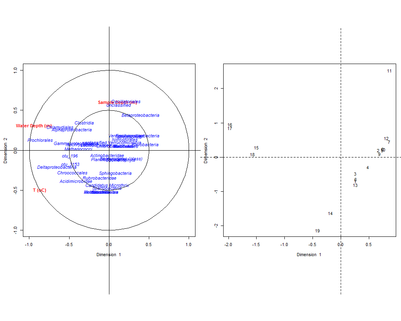
| − | [[Image:GOS3-CCA.png|thumb|center|401px|CCA Figure 3. | + | [[Image:GOS3-CCA.png|thumb|center|401px|CCA Figure 3. CCA output.]] |
===Step 4: Generate PEN and view in Cytoscape=== | ===Step 4: Generate PEN and view in Cytoscape=== | ||
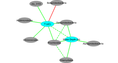
| − | [[GOS4-PENnetwork.png|thumb|center|401px|CCA Figure 4. | + | [[Image:GOS4-PENnetwork.png|thumb|center|401px|CCA Figure 4. Phenotype-environment network viewed in Cytoscape.]] |
==Dissimilarity Matrix Viewer== | ==Dissimilarity Matrix Viewer== | ||
Revision as of 00:34, 15 April 2013
GenGIS provides the following Python plugins which can be accessed through the Plugins menu.
Contents
Alpha Diversity
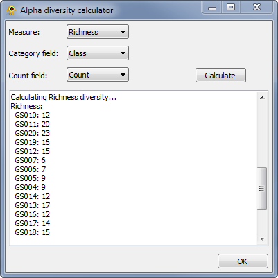
The Alpha Diversity plugin calculates alpha diversity for active locations. It currently calculate richness, Shannon, and Simpson alpha diversity. To calculate alpha diversity, you must select the Measure you wish to calculate and the Category field in your sequence file over which diversity will be calculate (Fig. 1). You may optionally select a Count field which indicates the number of times a given sequence is observed at a location. Pressing Calculate causes alpha diversity to be calculated. Results are reported within the plugin and added to the location table for use within GenGIS and other plugins.
Alpha Diversity Visualizer
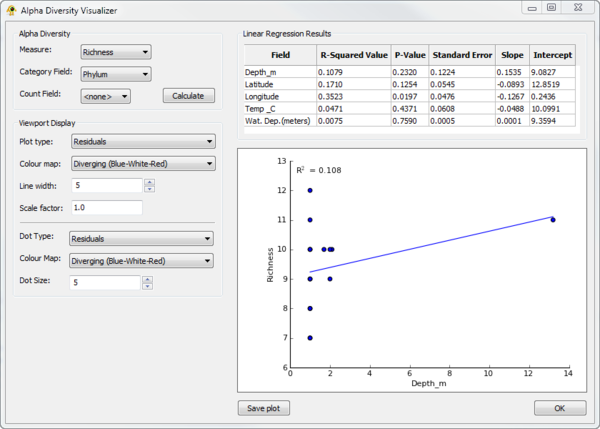
The Alpha Diversity Visualizer plugin can calculate alpha diversity for active locations, regress alpha diversity against location specific metadata, and produce visualizations of the resulting linear regression analysis. It currently calculate richness, Shannon, and Simpson alpha diversity. To calculate alpha diversity, you must select the Measure you wish to calculate and the Category field in your sequence file over which diversity will be calculate (Fig. 2). You may optionally select a Count field which indicates the number of times a given sequence is observed at a location. Pressing Calculate causes alpha diversity to be calculated. Linear regression results of alpha diversity versus all numeric fields associated with locations are reported within the Linear Regression Results table. Selecting a row within this table causes a linear regression scatter plot of alpha diversity versus the selected Field to be generated. The Viewport Display section allows different Viewport visualization to be produced.
Bar Graph
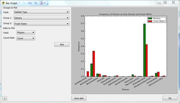
The Bar Graph plugin provides bar graphs showing the relative abundance of sequence data from two groups (Fig. 3). Groups can be defined be any field in your Location file and bar plots created for any numeric field in your Sequence file. You may optionally specify a Count field from the Sequence file indicates the number of times a given sequence is observed. This allows both qualitative and quantitative bar plots to be generated.
Beta Diversity Calculator
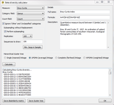
The Beta Diversity plugin calculates beta diversity between active locations (Fig. 4). The resulting biotic dissimilarity matrix can be saved to file and visualized in GenGIS using the Dissimilarity Matrix Viewer plugin. It currently calculate 9 measures of beta diversity (e.g., Bray-Curtis, Jaccard) across any field defined in your Sequence File. Sequences classified as Other or Unclassified can be optionally ignored during the calculation of beta diversity. In order to account for unequal sampling depth, subsampling with replacement (i.e., jackknifing) can be performed and the mean beta-diversity between jackknifed samples reported. Hierarchical cluster trees indicating the relative similarity of locations can be produced and used as an input Tree File to GenGIS.
Canonical Correlation Analysis
- Requirements: R with the cca library must be installed on your system (see the GenGIS manual).
The Canonical Correlation Analysis or CCA plugin implements the widely used statistical technique for joint analysis of biodiversity and environmental data across a number of sites. The plugin also generates Phenotype-Environment Network (PEN) graphs as described in Patel et al. (2010) Analysis of membrane proteins in metagenomics: Networks of correlated environmental features and protein families once a CCA has been carried out. The reference for the required R CCA package is Gonzalez et al (2008). The following example uses data from the Global Ocean Sampling dataset.
Step 1: Matrix Correlation
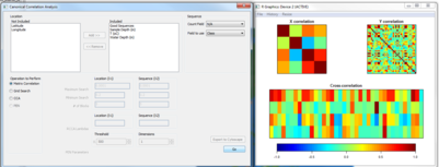
Before carrying out CCA, run the 'Matrix Correlation' function to ensure there is some level of correlation in the dataset. The figure below shows some evidence of strong and negative correlations, so we can proceed to the next step.
Step 2: Grid Search
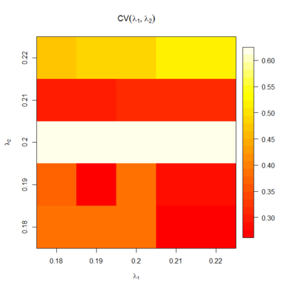
The cca library implements a grid search function to determine the optimum value of two key parameters, λ1 and λ2. To perform the grid search in reasonable time, we recommend starting with a coarse search (e.g., the default ranges as specified by the plugin) and iteratively seeking the best values by refining the parameters.
Step 3: Run CCA
Step 4: Generate PEN and view in Cytoscape
Dissimilarity Matrix Viewer
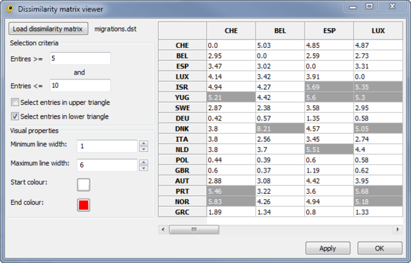
The Dissimilarity Matrix Viewer plugin provides functionality for visualizing a matrix which indicates the dissimilarity between all pairs of locations. The dissimilarity matrix must be in the following format, where a \t indicates a tab:
 3
A\t0\t2\t3
B\t1\t0\t4
C\t3\t5\t0
The first line indicates the number of locations and each of the following rows gives the dissimilarity values for the specified location. The location names (first column) must match those in your location file. The upper and lower triangles of the matrix can be different. For example, in this HIV-1 data set, the two triangle indicate import and export rates.
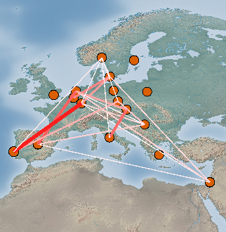
Elements in the matrix are selected by setting the Selection criteria (Fig. 5). Lines between the selected pairs are displayed in the Viewport using the specified Visual properties (Fig. 6). To update the Viewport display click Apply.
Linear Regression
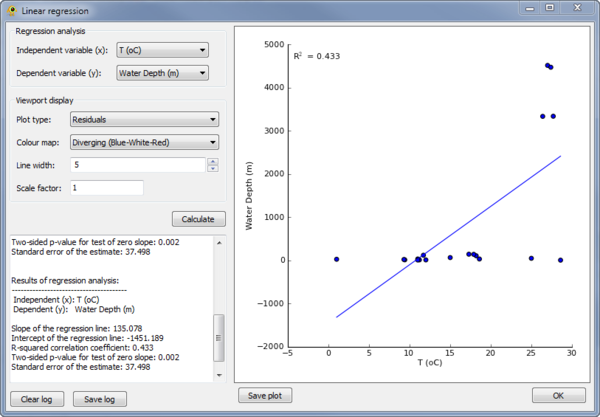
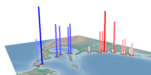
The Linear Regression plugin can be used to perform a linear regress between any two variables in the Location Table (see Location Table Viewer below). To perform the regression, the independent and dependent variables must be specified in the Regression analysis section of the plugin (Fig. 7). The results of the regression are reported within the plugin and shown as a scatter plot. A visualization within the GenGIS Viewport is also generated based on the properties set in the Viewport display section of the plugin (Fig. 8).
Location Table Viewer
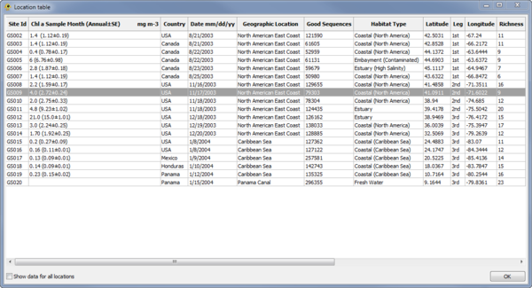
The Location Table Viewer plugin display a table indicating the metadata associated with each location (Fig. 9). Other plugins and custom Python scripts can be used to add data to the Location Table. By default, only data for active locations is shown. To show data for all locations check the Show data for all locations checkbox.
Mantel
- Requirements: R with the ade4 library must be installed on your system (see the GenGIS manual).
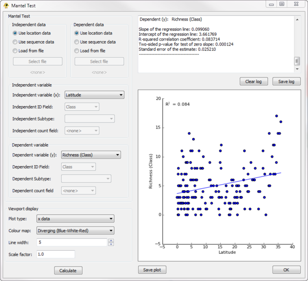
The Mantel plugin can be used to perform a Mantel test between any two variables in the Location Table or Sequence Table.
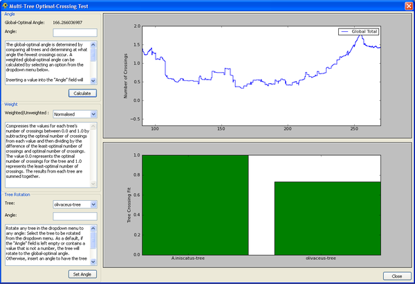
Multi-Tree Optimal-Crossing Test
Sequence Table Viewer
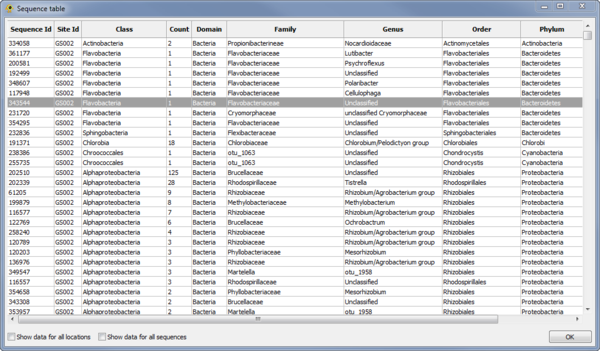
The Sequence Table Viewer plugin display a table indicating the metadata associated with each sequence (Fig. 12). Other plugins and custom Python scripts can be used to add data to the Sequence Table. By default, only data for active locations and active sequences is shown. To show data for all locations check the Show data for all locations checkbox. To show data for all sequences check the Show data for all sequences checkbox.
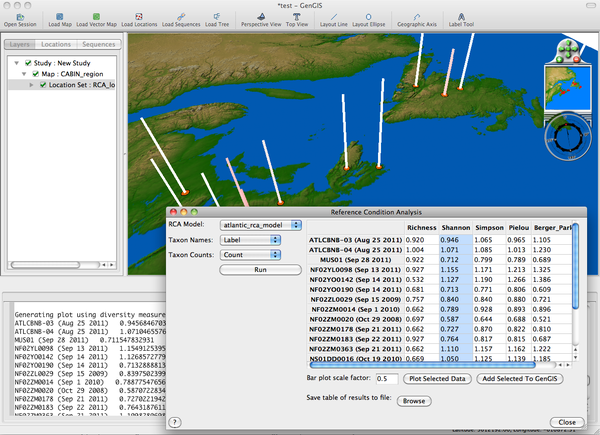
Reference Condition Analysis
- Overview:
- The Reference Condition Analysis plugin is used to evaluate impacts on biodiversity by computing the expected diversity based on several types of habitat metadata and compares these to the observed diversity.
- Requirements:
- R with the Vegan library must be installed on your system (see the GenGIS manual).
- Running RCA:
- Choose the appropriate RCA Model (currently only 'atlantic_rca_model' available). Select the appropriate data labels for Taxon Names and Taxon Counts.
- Browsing Results:
- The O/E (Observed over Expected diversity ratios) are displayed in the table for various alpha diversity measures including Richness, Shannon, Simpson, Pielou, and Berker-Parker.
- Each of these results can be plotted on the main GenGIS map by selecting a column in the table, optionally adjusting the "Bar plot scale factor", and clicking "Plot Selected Data".
- The data can be exported from the plugin table into GenGIS as another metadata habitat field allowing the use of other plugins (e.g. Linear Regression) by selecting a column and clicking "Add Selected To GenGIS".
- Lastly, the entire table of results can be saved to a tab-delimited file by using the "Browse" button.
