The GenGIS Manual
Welcome to the GenGIS manual. The sections below provide enough information to configure and start using GenGIS. Stay tuned for updates and send us your feedback when you get an opportunity.
Contents
Introduction / Overview of GenGIS
Purpose
Geography has always been an important component of evolutionary and ecological theory. The advent of sequence typing approaches such as 16S ribotyping, DNA barcoding using the COX1 gene, and multi-locus sequence typing, gives us the opportunity to understand how communities of organisms interact, move around and evolve. This sequencing revolution is tightly coupled to the development of new algorithms for assessing and comparing populations based on their genes.
Coupled with these developments is the ready availability of high quality, public domain digital map data. By integrating molecular data with cartography and habitat parameters, we can visualize the geographic and ecological factors that influence community composition and function.
GenGIS is designed to bring these components together into a single software package that satisfies the following criteria:
- Free and Open Source
- GenGIS is released under a Creative Commons Attribution - Share Alike 3.0 license, and we have made extensive use of other free packages such as wxWidgets, R, and Python. Making GenGIS freely available allows it to be downloaded and used anywhere in the world, and allows users to inspect and modify the source code.
- User-Friendly Interface
- Although GenGIS is built to deal with challenging scientific questions, our goal is to make the software as easy to use as possible. This is particularly important as many users will have little experience with digital map data, apart from applications such as Google Earth.
- Adaptible and Extensible
- The principal strength of many open-source projects lies in the ability of a loosely organized community of users to develop and enhance the software: R and BioPerl are two examples of successful open-source projects with many contributors. Since the potential applications of GenGIS are much broader than those we have in mind, we aim to make it as easy as possible to extend its capabilities by exposing the internal data structures and offering a plugin architecture.
Citing GenGIS
The best citation for GenGIS is indicated in boldface on the Main GenGIS page.
Where to Go for Help
- The latest version of the GenGIS manual (here).
- Text and video tutorials are available on the Tutorials page.
- The FAQ page keeps track of GenGIS-related questions.
- Please email beiko [at] cs.dal.ca with any questions or feedback about the software.
Installation
Getting the Latest Version of GenGIS
Download the latest version for Windows or Mac to get started visualizing and analyzing data in GenGIS.
Developer Version – building from source code
The source code for GenGIS is available on the Download page.
| Building on Windows | GenGIS can be compiled using Microsoft Visual C++ 2008 Express Edition. The Visual Studio solution file (GenGIS.sln) is located in the 'win32/build/msvc' directory. Please note that the built-in Python console is only available in Release builds. |
|---|---|
| Building on MacOSX | GenGIS can be compiled using the Makefile located in the 'mac/build/gcc' directory. To compile, simply run 'make release' within a terminal. Development has been performed using the gcc 4.3.3 compiler. |
System Requirements
GenGIS has been developed and tested on the following operating systems:
- Windows (XP, Vista & 7) 32-bit binaries compatible with 64-bit Windows releases.
- Mac OS X (v10.5 'Leopard' & v10.6 'Snow Leopard') Intel-based only
Support for Linux is not a development priority at this time. Porting to Linux should be a fairly straightforward operation as GenGIS has been developed using cross-platform libraries. Efforts to port GenGIS to other operating systems are encouraged. As always, your feedback on this project is greatly appreciated.
Input data
File Types
GenGIS works with four different types of data files:
- Digital Map File (sample)
- Location File (sample)
- Sequence File (sample)
- Phylogenetic Tree File (sample)
To start working with GenGIS, first load the Digital Map file followed by the Location file. Once these files are loaded, any number of Sequence and/or Phylogenetic Tree files can be opened.
A Technical Note: The location of sequences (Sequence file) and leaves (Phylogenetic Tree file) must each map to an existing location given by the Location file.
Maps
GenGIS relies on the Geospatial Data Abstraction Library (GDAL) to import several digital map file formats and projections. More information, including community support and downloads, can be found at the GDAL website.
A Technical Note: The 'gdal_merge.py' script, 'gdalwarp.exe' and 'gdal_translate.exe' executables have been very useful in preparing maps compatible with GenGIS.
Supported formats
GenGIS supports the formats listed on the GDAL Raster Formats page. Note that not all formats have been tested at this time. The following formats have been found to work reliably:
- GeoTIFF
- Arc/Info ASCIIGRID
- USGS DEM (and variations thereof)
Projections
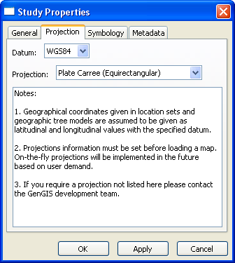
If you wish to use a specific projection, you must specify it before loading your map - GenGIS is unable to render reprojections on the fly. This is particularly true if you are loading the default world map (from GTOPO30) that ships with GenGIS: the default Mercator projection stretches the polar regions, whereas Plate Carre or Robinson will provide a much less distorted world view.
To specify the projection before loading the map, right click "New Study : Study" in the Layers tab, and select Properties. Selecting the Projection tab will allow you to choose your projection.
GenGIS currently does not support projections in which a single point is displayed in multiple locations. The best example of this is the default world map, which is modified to stretch from 89.9 degrees North to 89.9 degrees South latitude. Since the poles stretch across the entire upper and lower edges of a map in a projection such as Plate Carre, GenGIS is unable to display these properly.
Typical limits on map size
Higher processor speeds and more system RAM are required to work effectively with larger maps. Typically one gigabyte of RAM permits working with maps that are 10 megabytes or slightly greater in size.
Reducing Map Size
If the map resolution of is too high for the system hardware being used, the GDAL Utilities 'gdalwarp' or 'gdal_translate' can be used to reduce the density of points in the map. Decreasing the level of detail is an acceptable tradeoff in many cases.
Location File
The location file must be provided in a comma-separated format (e.g., the .CSV files that can be exported from Microsoft Excel). The first line of the file must be a comma-separated series of headers. Each subsequent line will contain a set of attributes for a single location.
The first three entries on each line must be:
- A unique location identifier
- A vertical coordinate, either decimal degrees of latitude or Universal Transverse Mercator (UTM) northing. Note that positive values = north and negative values = south.
- A horizontal coordinate, either decimal degrees of longitude or UTM easting. Positive values = east and negative values = west.
The first line of the file must therefore begin with the following three column headings:
Site ID,Latitude,Longitude
or
Site ID,Northing,Easting
depending on the coordinate system.
After these three columns, you can specify anything you like in the Location file, including longer descriptive site names, environmental parameters, and a time stamp. So, for instance, a location file header might look like this:
Site ID,Latitude,Longitude,File Size,Environment Type,Geographic Location,Site Name,Country
Each of these values must then be specified for every entity (= row in the file), even if they are called NULL or some other placeholder value.
Sequence File
The basic specification of the sequence file is even simpler, with only two required fields:
- A unique location identifier that is also found in the location file
- A unique sequence identifier
The first line of the file must begin with the following column headings:
Site ID, Sequence ID
As with the location file, columns containing custom information can be added after the two mandatory headings. Each row of the sequence file must define a value for each of the columns identified in the header line. Note that the 'sequence file' need not contain any molecular sequence data, nor do the entities necessarily need to have a one-to-one correspondence to actual sampled sequences.
A simple sequence file might summarize the taxonomic classification of each sampled sequence:
Site ID,Sequence ID,Best_match,Species,Genus,Family,Order,Class,Phylum,Superkingdom
Phylogenetic trees
Input phylogenetic trees should adhere to the Newick file format, with the additional constraint that leaf labels must match up exactly with either a Site ID from the location file or a Sequence ID from the sequence file.
The Environment
Overview
|
|
|
|
| |
|
|
| |
Menu Items
|
|
Toolbar Buttons
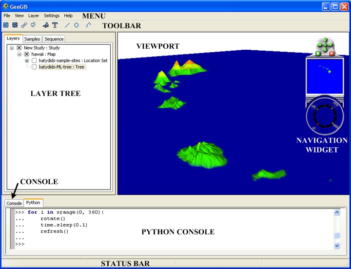
The Toolbar provides easy access to frequently used features.
| Add map | Add a map to the currently selected study. | |
| Add location set | Add a location set to the currently selected map. | |
| Add sequence data | Add sequence data to the currently selected location set. | |
| Add tree | Add a geographic tree model to the currently selected map. | |
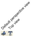
| Default perspective view | Move camera to its default perspective position. | |
| Top view | Move camera to give a top-down view of the map. | |
| Draw layout line | Draw a straight line which can be used to layout graphic elements such as a 2D tree or pie charts. | |
| Draw layout ellipse | Draw an ellipse which can be used to layout graphic elements such as a 2D tree or pie charts. | |
| Draw geographic axis | Draw a polyline which can be used to test the goodness-of-fit between a tree and a non-linear geographic axes (see 2D Pylogenetic Trees). |
Note: Adding multiple location sets, sequence sets or trees is experimental at this time. GenGIS does not support loading multiple maps.
Layer Tree Controller
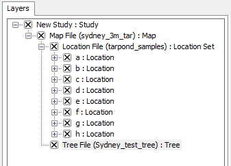
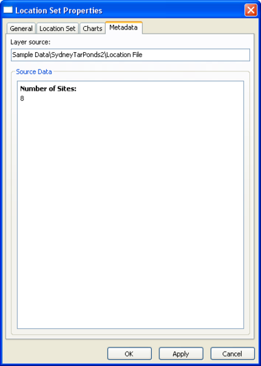
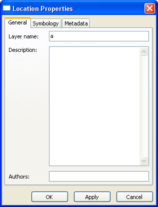
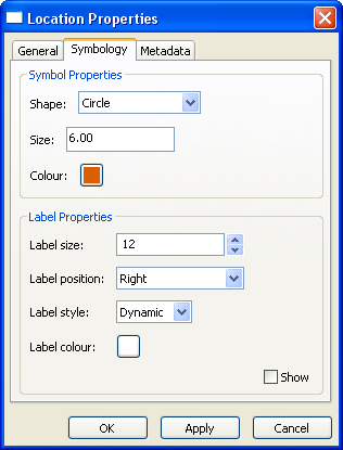
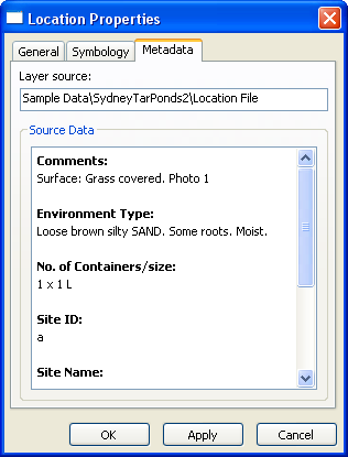
| The Layer Tree Controller is located in the left panel within GenGIS and provides a hierarchical view of the Study, Map, Location Set, Location, Sequence and Tree layers.
Double clicking (or right clicking and selecting 'Properties' from the pop-up menu) on the text region of any layer title brings up the properties dialog for that layer. Layers can be enabled (shown) and disabled (hidden) in the viewport window by clicking the 'x' boxes to the left of each layer name. |
Console Panels
Console
Python Console
Interacting with sample sites
Layer Property Dialogs
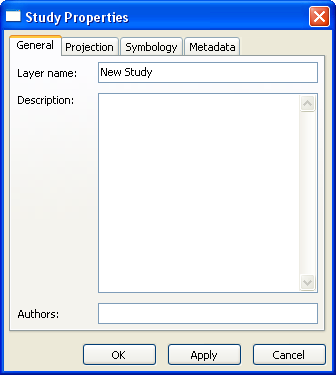
Study Layer Properties
|
| ||||
|
|
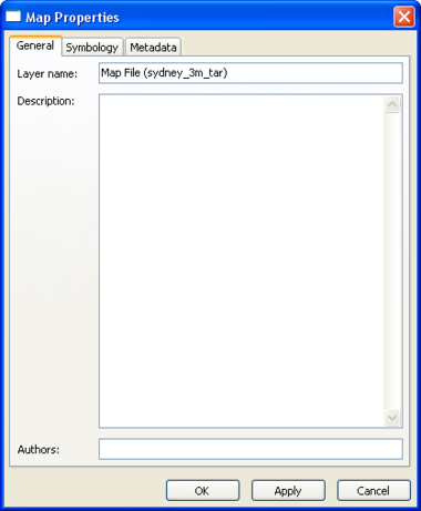
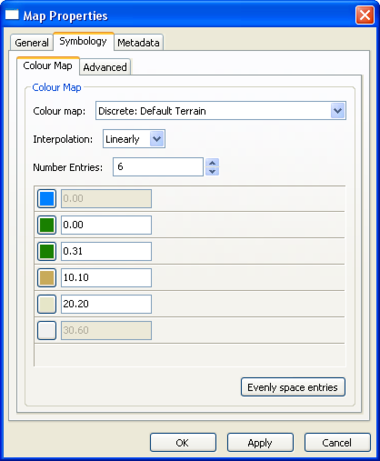
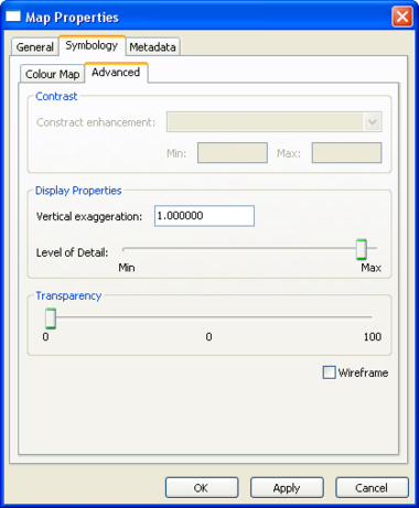
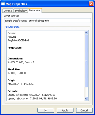
Map Layer Properties
|
| ||||
|
|
|
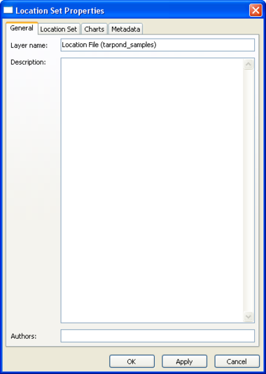
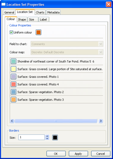
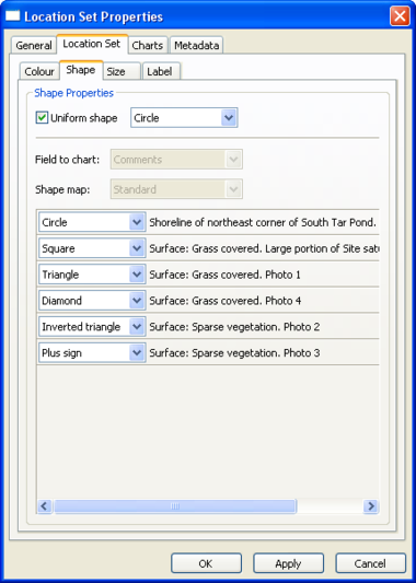
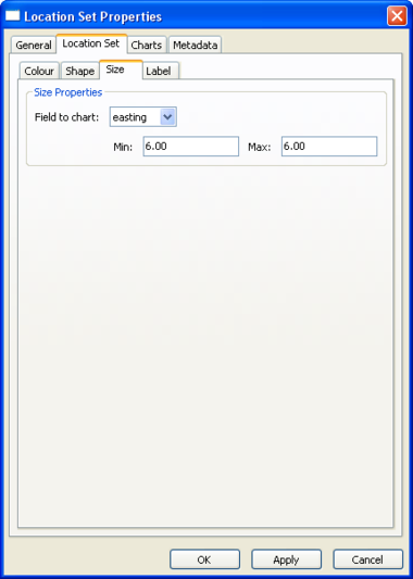
Location Set Layer Properties
|
|
| ||||
|
|
| ||||
|
|
| ||||
|
|
| ||||
|
|
|
Location Layer Properties
|
|
| ||||
|
|
|
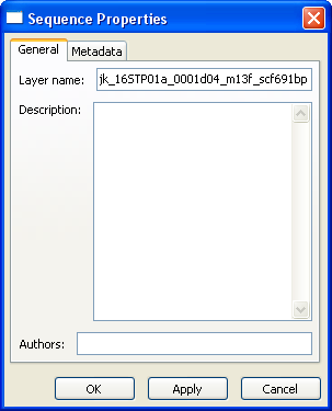
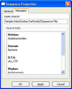
Sequence Layer Properties
|
|
|
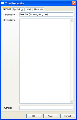
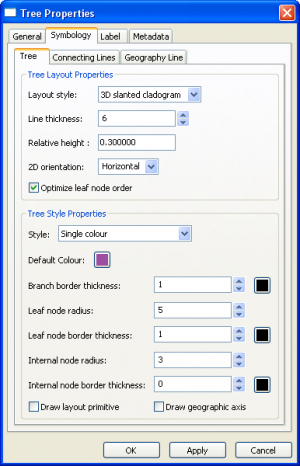
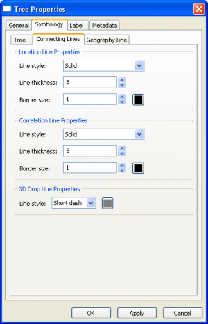
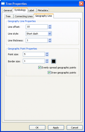
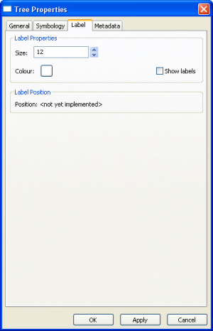
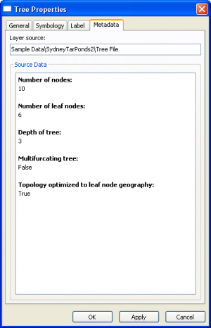
Tree Layer Properties
|
|
| ||||
|
|
| ||||
|
|
|
Graphical analysis tools in GenGIS
Basic data visualizations
Pie charts
2D phylogenetic trees
Coming soon!
The algorithm to layout a 2D tree has an exponential running time in the degree of a node. As such, we do not suggest trying to layout trees with nodes of degree > 10. Details of this algorithm are given in:
Parks, D.H. and Beiko, R.G. (2009). Quantitative visualizations of hierarchically organized data in a geographic context. Accepted to Geoinformatics 2009, Fairfax, VA.
Defining axes
Manipulation
3D phylogenetic trees
The Python console and API functions
What you can do with the console
The Python Console provides access to a standard Python interpreter. Python is a general-purpose high-level programming language with many packages available for phylogenetics, population genetics, and statistics. Data loaded into GenGIS is exposed to the Python Console allowing quanitative hypothesis testing to be performed directly within GenGIS. Results of analyses can be visualized within the Viewport to aid in interpretation of results and generation of new hypotheses.
Here is a list of all API functions. Below we give several short examples of using this API. You can also find information about using the API on our tutorials page.
Accessing location site and sequence data
Location site and sequence data can be accessed directly from the Python Console. The easiest way to do this is to utilize functions within the dataHelper.py file located in your scripts directory. To make use of these functions they must first be imported:
import dataHelper
You can access location data using:
locData = dataHelper.getLocationSetData()
This will read in the location data from the first location set under the first map in the Layer Tree. Location data is returned as a Python list of location objects. Location objects contain a number of functions along with a Python dictionary holding all metadata associated with the location:
temp = locData[0].data['Temperature']
To access location set data from the 2nd location set under the 3rd map use:
locData = dataHelper.getLocationSetData(2, 3)
Sequence data is accessed in an analogous manner:
seqData = dataHelper.getSequenceData()
Sequence data is returned as a Python list of sequence objects. Sequence objects contain a Python dictionary of all metadata associated with a sequence:
phylum = seqData[0].data['Phylum']
To get sequence data from the ith location of the jth location set of the kth map use:
seqData = dataHelper.getSequenceData(i, j, k)
If you wish to understand the low-level details on how to access data please consult the functions in dataHelper.py. We plan to extend the dataHelper interface in the future to allow data to be queried by name in addition to being queried by index position.
Filtering data
We have provided a simple function, filterData, for filtering data. This function is contained in dataHelper.py. As an example, all locations with a temperature greater than 20 can be obtained as follows:
import dataHelper
locData = dataHelper.getLocationSetData()
filteredData = dataHelper.filterData(locData, 'Temperature', 20, dataHelper.filterFunc.greater)
The function filterData takes 4 parameters:
- the data to be filtered
- the field to filter on
- the value to filter on
- a filtering function which returns true for all items passing the filter
Filtering can be done on either strings or numeric values:
import dataHelper
seqData = dataHelper.getSequenceData()
filteredData = dataHelper.filterData(seqData, 'Phylum', 'Actinobacteria', dataHelper.filterFunc.equal)
Basic filtering functions are provided in filterFunc.py, but it is easy to write your own filtering functions. For example, the equal filter used above is simply:
def equal(val1, val2):
  return str(val1) == str(val2)
Selecting sequences
GenGIS supports the notion of an active set of sequences. Calculations and visualizations reflect only those sequences in the active set. You can add or remove sequences from the active set using the SetActive member function. As an example, one could select only those sequences classified as Gammaproteobacteria, Betaproteobacteria, or Epsilonproteobacteria in order to produce pie charts showing the relative proportion of sequences from these three classes:
seqData = dataHelper.getSequenceData()
for seq in seqData:
  if seq.data['Class'] in ['Gammaproteobacteria', 'Betaproteobacteria', 'Epsilonproteobacteria']:
    seq.SetActive(True)
  else:
    seq.SetActive(False)
dataHelper.getChartSetView().UpdateCharts()
refresh()
You can also use the helper function selectData to place sequences into the active set:
import dataHelper
seqData = dataHelper.getSequenceData()
dataHelper.selectData(seqData, 'Phylum', 'Actinobacteria', dataHelper.filterFunc.equal)
The helper function selectAllSeqs can be used to place all sequences into the active set:
seqData = dataHelper.getSequenceData()
dataHelper.selectAllSeqs(seqData)
Creating custom data visualizations
Using the VisualLine, VisualMarker, and VisualLabel classes one can create custom data visualizations with GenGIS. The VisualLine class allows user defined lines to be drawn in the Viewport. Suppose we have two locations within our location set with ids of 'GBR' and 'ITA'. We can draw a line between these locations as follows:
# get location data
import dataHelper as dh
locData = dh.getLocationSetData()
# create a dictionary indicating the geographic coordinates of each location
locDict = {}
for loc in locData:
  locDict[loc.id] = [loc.northing, loc.easting]

# get the 3D position of GBR and ITA
gbrPt = Point3D()
convertGeoCoord(locDict['GBR'][0], locDict['GBR'][1], gbrPt)
itaPt = Point3D()
convertGeoCoord(locDict['ITA'][0], locDict['ITA'][1], itaPt)
# draw a solid red line with a width of 2 between these countries
line = VisualLine(Colour(1,0,0), 2, LINE_STYLE.SOLID, Line3D(gbrPt, itaPt))
lineId = addLine(line)
refresh()
The visual properties of this line can easily be changed at any time to reflect different aspects of your data:
line.SetColour(Colour(1,0,1))
line.SetSize(5)
line.SetLineStyle(LINE_STYLE.SHORT_DASH)
refresh()
We can later remove this line using:
removeLine(lineId)
The VisualMarker class allows user defined markers to be drawn in the Viewport. It is similar to the VisualLine class. For example, we can draw a blue circle over London which is situated at a latitude of 51.51N and a longitude 0.128W as follows:
# get 3D position of geographic coordinate in Viewport
pt = Point3D()
convertLatLong(51.51, -0.128, pt)
marker = VisualMarker(Colour(0,0,1), 6, MARKER_SHAPE.CIRCLE, pt)
markerId = addMarker(marker)
refresh()
VisualLabels can be used to create orthographic (e.g., to indicate a legend or figure caption) or perspective text (e.g., to label points on a map). We can create a "Hello World!" label for a map as follows:
label = VisualLabel("Hello World!", Colour(0,0,0), 12)
label.SetScreenPosition(Point3D(20,20,1))
label.SetRenderingStyle(LABEL_RENDERING_STYLE.ORTHO)
labelId = addLabel(label)
refresh()
Alternatively, we can use a VisualLabel to label our marker at London:
label = VisualLabel("London", Colour(0,0,0), 12)
pt = Point3D()
convertLatLong(51.51, -0.128, pt)
label.SetGridPosition(pt)
label.SetRenderingStyle(LABEL_RENDERING_STYLE.PERSPECTIVE)
labelId = addLabel(label)
refresh()
By combining these graphical primative and encoding key aspects of your data to different visual properties (i.e., colour, size, shape) GenGIS can be used to identify interesting patterns within a wide-range of datasets. An example which uses these classes to visualizing a distance matrix indicating the rate of import and export of HIV-1 subtype B for different European countries as reported by Paraskevis et al. (2009) is available here.
Creating fly-through movies
A collection of functions for creating fly-through movies are available in movieHelper.py found in the scripts directory. A useful movie is to rotate the map about its origin. Such a movie can be made using the rotateAboutOrigin function which takes the number of degrees to rotate and the time of the movie as parameters:
import movieHelper
movieHelper.rotateAboutOrigin(360, 10)
More general movies can be created by capturing the camera parameters at key frames using the function getCameraParam and then interpolating between these key frames using the function linearInterpolateParams:
import movieHelper
# move camera to first key frame (for example, use the toolbar to set a top down view)
keyFrame1 = movieHelper.getCameraParam()
# move camera to next key frame (for example, use the toolbar to set the default perspective view)
keyFrame2 = movieHelper.getCameraParam()
# set camera back to first key frame
movieHelper.setCameraParam(keyFrame1)
# smoothly move between these key frames in 5 seconds
movieHelper.linearInterpolateParams(keyFrame1, keyFrame2, 5)
For examples of creating custom movies which do not use the movieHelper API, have a look at the series of H1N1 movies we have developed. In particular, note that wxSafeYield must be called occasionally for time series to run correctly.
By stitching together multiple key frames complex fly-through movies can be created. Commercial software such as Camtasia or open source software such as CamStudio can be used to record these movies.
