Description of GenGIS plugins
GenGIS provides the following Python plugins which can be accessed through the Data and Plugins menus. Please contact us if you have questions about using the plugins, or if you have suggestions for new plugins.
Contents
- 1 Data Retrieval
- 2 Analysis Plugins
- 2.1 Alpha Diversity
- 2.2 Alpha Diversity Visualizer
- 2.3 Bar Graph
- 2.4 Beta Diversity Calculator
- 2.5 Canonical Correlation Analysis
- 2.6 Dissimilarity Matrix Viewer
- 2.7 Environmental Data Visualizer
- 2.8 Linear Regression
- 2.9 Location Table Viewer
- 2.10 Mantel Test
- 2.11 Multi-Tree Optimal-Crossing Test
- 2.12 Sequence Table Viewer
- 2.13 Reference Condition Analysis
- 2.14 Show Spread
Data Retrieval
We are currently developing plugins to retrieve data from several online sources. In all cases, we ask that you familiarize yourself with the relevant Terms of Use and any Disclaimers regarding use of the data; we link to these below wherever possible. The developers of GenGIS are in no way responsible for data provided by third-party sources, and are not liable for any consequences arising from the use of our software and plugins.
GBIF Query
The GBIF Query plugin creates location and sequence data for use in GenGIS from the Global Biodiversity Information Facility (GBIF). It queries the GBIF database with one or more user-provided taxon names and a geographic range, and returns all instances with geographic location data that match the query. When using the GBIF plugin to create datasets, please read and adhere to GBIF's Data Use Agreement and Data Sharing Agreements. Our plugin makes use of the GBIF public API, which is still somewhat in flux - please let us know if you encounter any problems.
For the purposes of the next example, it is assumed that the user has loaded a Raster Map file. If a user has not loaded a Raster Map then Add Data will not be available, but the retrieved data can still be saved to disk.
Please be aware that large queries may result in the plugin entering a Not Responding state. This is controlled by the operating system, and while the plugin will not respond to user input, it is still performing its query.
Furthermore there may be cases where the count returned from Query Records may not exactly match the amount of records returned from the plugin. This is because GBIF occasionally will return results slightly outside of a specified range. To procure these samples as well it is often enough to adjust the geographic border to the next largest integer.
Step 1: The Query
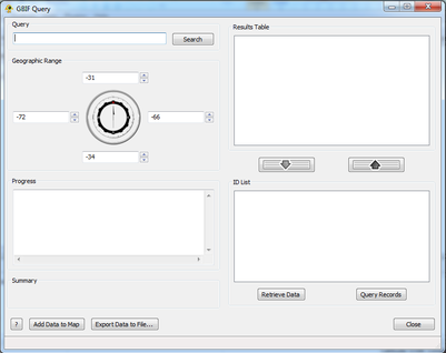
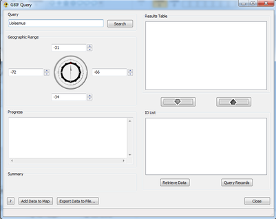
In order to query GBIF two things must be entered: a taxon name and a geographic range. If a map is loaded prior to running this plugin the default range borders will be the extents of the map; if not they will be the entire world. The geographic range can be fine tuned using either text input or the scroll wheels. After the appropriate information has been entered hitting Search will query GBIF for all possible taxonomic matches.
Step 2: Add/Remove Items
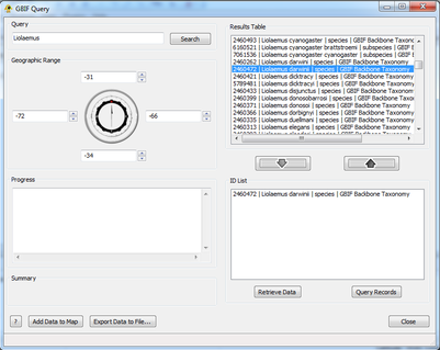
Hitting Search populates the Results Table. This is where all matches are returned by GBIF:
Unique ID Number | Full Name | Biological Classification | Data Source
Highlighting entries in this list and clicking Add or double-clicking entries adds them to the ID List. This list is what will be used to query GBIF to create the location and sequence file. Highlighting an entry in this list and clicking Remove or double-clicking an entry removes it from consideration. A user can perform multiple queries and add multiple taxa to this list, but only one geographic range can be defined.
Step 3: Retrieve Data/Query Records
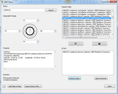
Once the user is satisfied with the contents of the ID List they can choose either Retrieve Data or Query Records. Query Records quickly retrieves the number of results without retrieving the results themselves; this can be used to quickly determine whether the size of the data set will be suitable for use in GenGIS. This information is displayed in the Summary dialog box. Large data sets (e.g., >1000 locations) will take more time to retrieve and process, as well as slow down GenGIS. If the user is satisfied with the amount of records they are about to retrieve they can move on to the Retrieve Data option. Here GBIF is queried and the progress of that query is displayed in the Progress box.
Step 4: Add/Export Data
Finally the user can choose to export their data to a location on their disk drive, or add it directly to GenGIS. The Export button writes three separate files to a user-specified location on disk. These files are the location file, sequence file and a source file containing collection metadata for the data set, any specialized rights associated with that data, and how to cite them for published works. Saving data in files eliminates the need to redo lengthy queries at a later date. If Add Data is selected then the location and sequence files are added directly to GenGIS without saving. The source information is imported into the description of the location layer.
MG-RAST Query
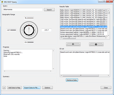
The MG-RAST Query plugin creates location and sequence data for use in GenGIS from the RAST (MG-RAST) Server. It queries the MG-RAST database with a user-provided organism or function located within a geographic range and returns contents of associated studies to be used in GenGIS.
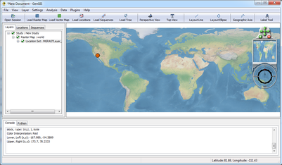
For the purposes of the next example, it is assumed that the user has loaded a Raster Map file. If a user has not loaded a Raster Map then Add Data will not be available, but the retrieved data can still be saved to disk.
Please be aware that large queries may result in the plugin entering a Not Responding state. This is controlled by the operating system, and while the plugin will not respond to user input, it is still performing its query. Also, the MG-RAST service has occasional periods where it is not available, which will generate errors when using the GenGIS plugin.
Step 1: The Query
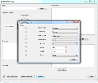
The MG-RAST Query plugin can search MG-RAST for studies based upon organism name or function. Alternatively, studies can be retrieved directly by searching the corresponding ID. This can be selected from the Options button highlighted below.
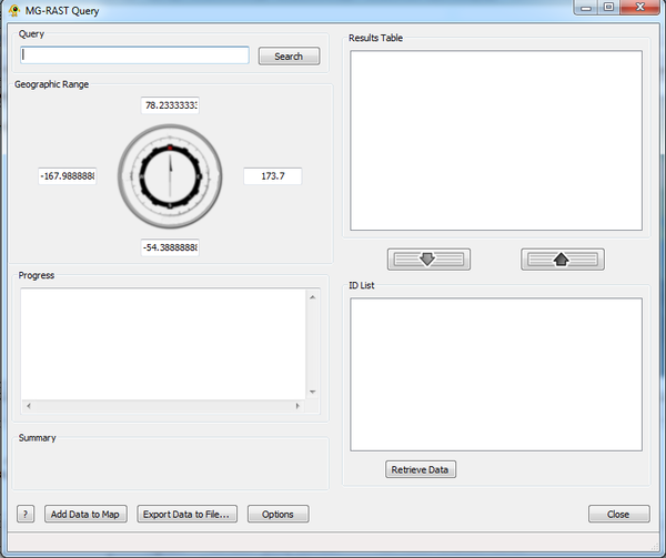
In order to query MG-RAST two things must be entered: a taxon name and a geographic range. If a map is loaded prior to running this plugin the default range borders will be the extents of the map, if not they will be the entire world (lat:-90,90 lon:-180,180). The geographic range can be fine tuned using either text input. After the appropriate information has been entered hitting Search will query MG-RAST for all possible matches. This functionality can be overridden if the user has selected Study as their search type. Doing this will allow them to directly input a study ID to download. Hitting Search in this case will retrieve that study from MG-RAST immediately, shortcutting all other steps. Multiple studies can be queried at once but entering them in the search field separated by a single space character.
Step 2: Add/Remove Items
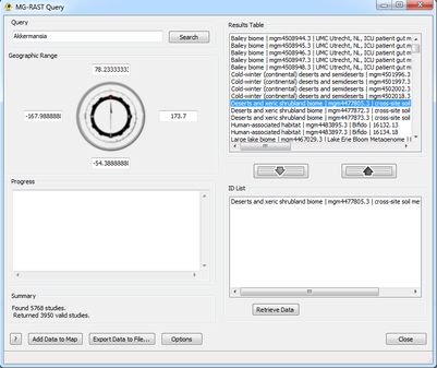
Hitting Search populates the Results Table. This is where all matches are returned by MG-RAST:
Unique ID Number | Study Name | Project Name
Highlighting entries in this list and clicking Add or double-clicking entries adds them to the ID List. This list is what will be used to query MG-RAST to create the location and sequence file. Highlighting an entry in this list and clicking Remove or double-clicking an entry removes it from consideration. A user can perform multiple queries and add multiple taxa to this list, but only one geographic range can be defined.
Step 3: Retrieve Data/Query Records
Once the user is satisfied with the contents of the ID List they can choose either to customize their search or to Retrieve Data. To customize the search click the Options buttons and select any relevant fields and settings. These will be appended to the query. For more information as to the function of these fields please refer to [1]. Retrieve Data will query MG-RAST with the specified options and display the progress of that query in the Progress box. Note that MG-RAST datasets are typically large, and the retrieval process may take a while.
Step 4: Add/Export Data
Finally the user can choose to export their data to a location on their disk drive, or add it directly to GenGIS. The Export button writes two separate files to a user-specified location on disk. These files are the location file, sequence file. Saving data in files eliminates the need to redo lengthy queries at a later date. If Add Data is selected then the location and sequence files are added directly to GenGIS without saving. The user can then choose to save the session, but can no longer save the location and source information separately.
Worldclim Query
The WorldClim Query plugin adds environmental information to location data. This plugin adds data acquired by WorldClim (www.worldclim.org) to Latitude/Longitude associated locations through a Python module called Pybioclim. This module has a granularity of 0.083 degrees by 0.083 degrees. If two or more data points are closer together, they will be assigned the same values.
Due to the necessity of Latitude/Longitude based coordinates, if not projection is available your map/data will not be compatible with this plugin.
Only Map and Location data is necessary for this Plugin to work. Sequence data is optional.
Set 1: The Query
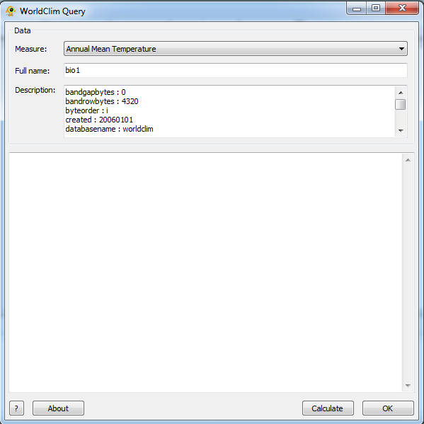
The WorlClim Query plugin offers nineteen different environmental fields to choose from. These are essentially divided into two different types of data: Temperature information and Precipitation information. To select a different environmental data, choose from the Measure drop down. When a measure is selected the Name and Description field will be populated with the relevant information pertaining to the selected measure.
This is the only required field to perform a query.
Step 2: Calculate
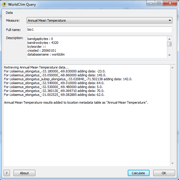
Once the appropriate measure has been selected hit the Calculate button on the lower right of the plugin. This will retrieve the selected measure information for each location.
Analysis Plugins
Alpha Diversity
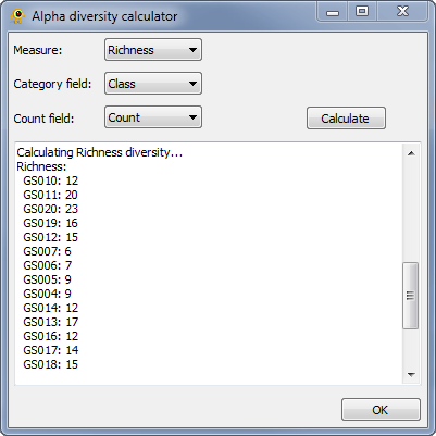
The Alpha Diversity plugin calculates alpha diversity for active locations. It currently calculate richness, Shannon, and Simpson alpha diversity. To calculate alpha diversity, you must select the Measure you wish to calculate and the Category field in your sequence file over which diversity will be calculated. You may optionally select a Count field which indicates the number of times a given sequence is observed at a location. Pressing Calculate causes alpha diversity to be calculated. Results are reported within the plugin and added to the location table for use within GenGIS and other plugins.
Alpha Diversity Visualizer
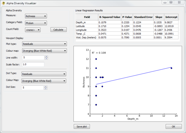
The Alpha Diversity Visualizer plugin can calculate alpha diversity for active locations, regress alpha diversity against location specific metadata, and produce visualizations of the resulting linear regression analysis. It currently calculate richness, Shannon, and Simpson alpha diversity. To calculate alpha diversity, you must select the Measure you wish to calculate and the Category field in your sequence file over which diversity will be calculated. You may optionally select a Count field which indicates the number of times a given sequence is observed at a location. Pressing Calculate causes alpha diversity to be calculated. Linear regression results of alpha diversity versus all numeric fields associated with locations are reported within the Linear Regression Results table. Selecting a row within this table causes a linear regression scatter plot of alpha diversity versus the selected Field to be generated. The Viewport Display section allows different Viewport visualization to be produced.
Bar Graph
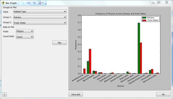
The Bar Graph plugin provides bar graphs showing the relative abundance of sequence data from two groups. Groups can be defined be any field in your Location file and bar plots created for any numeric field in your Sequence file. You may optionally specify a Count field from the Sequence file indicates the number of times a given sequence is observed. This allows both qualitative and quantitative bar plots to be generated.
Beta Diversity Calculator
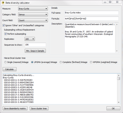
The Beta Diversity plugin calculates beta diversity between active locations. The resulting biotic dissimilarity matrix can be saved to file and visualized in GenGIS using the Dissimilarity Matrix Viewer plugin. It currently calculate 9 measures of beta diversity (e.g., Bray-Curtis, Jaccard) across any field defined in your Sequence File. Sequences classified as Other or Unclassified can be optionally ignored during the calculation of beta diversity. In order to account for unequal sampling depth, subsampling with replacement (i.e., jackknifing) can be performed and the mean beta-diversity between jackknifed samples reported. Hierarchical cluster trees indicating the relative similarity of locations can be produced and used as an input Tree File to GenGIS.
Canonical Correlation Analysis
- Requirements: R with the cca library must be installed on your system (see the GenGIS manual).
The Canonical Correlation Analysis or CCA plugin implements the widely used statistical technique for joint analysis of biodiversity and environmental data across a number of sites. The plugin also generates Phenotype-Environment Network (PEN) graphs as described in Patel et al. (2010) Analysis of membrane proteins in metagenomics: Networks of correlated environmental features and protein families once a CCA has been carried out. The reference for the required R CCA package is Gonzalez et al (2008). The following example uses data from the Global Ocean Sampling dataset.
Step 1: Matrix Correlation
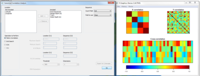
Before carrying out CCA, run the 'Matrix Correlation' function to ensure there is some level of correlation in the dataset. The figure below shows some evidence of strong and negative correlations, so we can proceed to the next step.
Step 2: Grid Search
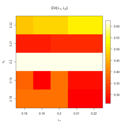
The cca library implements a grid search function to determine the optimum value of two key parameters, λ1 and λ2. To perform the grid search in reasonable time, we recommend starting with a coarse search (e.g., the default ranges as specified by the plugin) and iteratively seeking the best values by refining the parameters.
Step 3: Run CCA
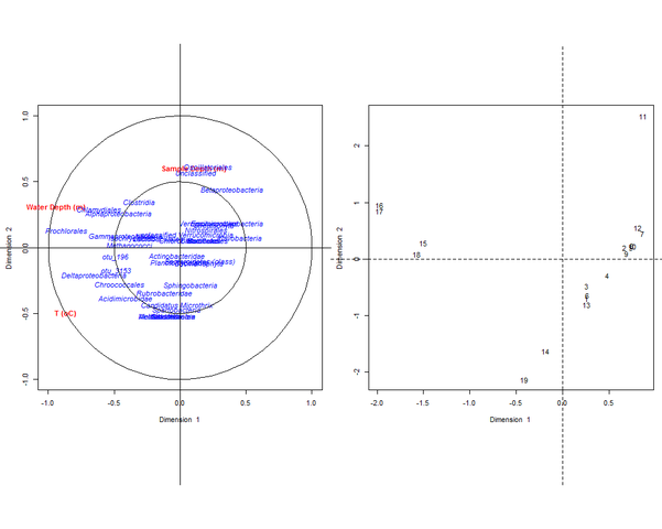
After choosing the most appropriate values of λ1 and λ2, we run the CCA to generate biplots that show the relationships between our input habitat and sequence count variables. The abundance of certain taxonomic classes seems to correlate with the three environmental variables considered.
Step 4: Generate PEN and view in Cytoscape
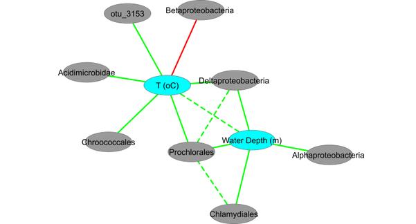
To gain a better perspective on the relationships between variables, we can generate a phenotype-environment network that displays each variable as a node, and connects nodes for which the products of canonical correlates for the chosen number of dimensions sum to an absolute value greater than the chosen threshold. The network below, exported as a .xgmml file and imported into Cytoscape, shows relationships based on the first two dimensions, with positive correlations in green and negative ones in red.
Dissimilarity Matrix Viewer
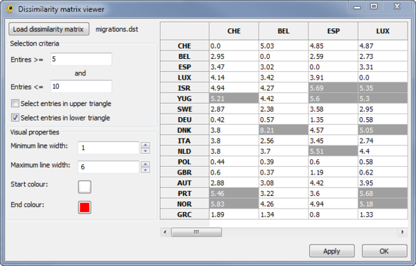
The Dissimilarity Matrix Viewer plugin provides functionality for visualizing a matrix which indicates the dissimilarity between all pairs of locations. The dissimilarity matrix must be in the following format, where a \t indicates a tab:
 3
A\t0\t2\t3
B\t1\t0\t4
C\t3\t5\t0
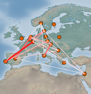
The first line indicates the number of locations and each of the following rows gives the dissimilarity values for the specified location. The location names (first column) must match those in your location file. The upper and lower triangles of the matrix can be different. For example, in this HIV-1 data set, the two triangle indicate import and export rates.
Elements in the matrix are selected by setting the Selection criteria.
Lines between the selected pairs are displayed in the Viewport using the specified Visual properties. To update the Viewport display click Apply.
Environmental Data Visualizer
Under construction - for 2.11 release
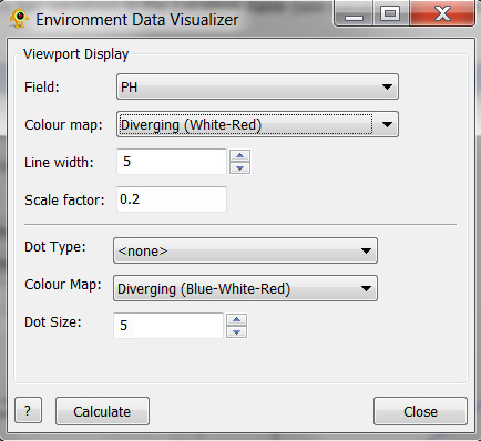
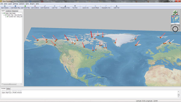
The Environmental Data Visualizer plugin displays environmental data as bar graphs and colored points on a map, in a manner similar to the Alpha Diversity Visualizer plugin but without the need for sequence data to be loaded or defined.
Linear Regression
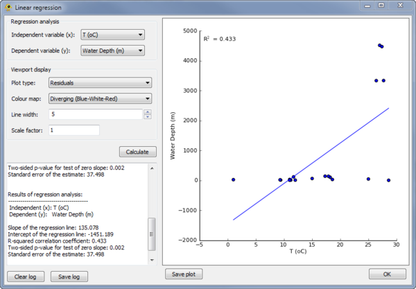
The Linear Regression plugin can be used to perform a linear regress between any two variables in the Location Table (see Location Table Viewer below). To perform the regression, the independent and dependent variables must be specified in the Regression analysis section of the plugin.
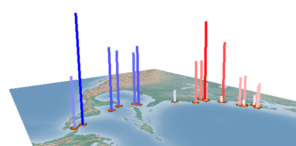
The results of the regression are reported within the plugin and shown as a scatter plot. A visualization within the GenGIS Viewport is also generated based on the properties set in the Viewport display section of the plugin.
Location Table Viewer
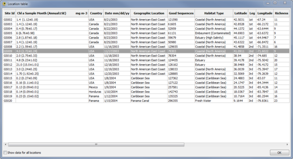
The Location Table Viewer plugin display a table indicating the metadata associated with each location. Other plugins and custom Python scripts can be used to add data to the Location Table. By default, only data for active locations is shown. To show data for all locations check the Show data for all locations checkbox.
Mantel Test
- Requirements: R with the ade4 library must be installed on your system (see the GenGIS manual).
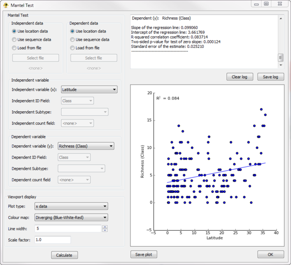
The Mantel plugin can be used to perform a Mantel test between any two variables in the Location Table or Sequence Table.
Multi-Tree Optimal-Crossing Test
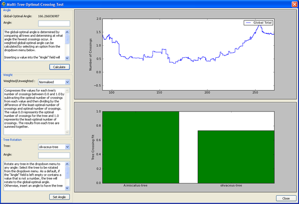
This plugin will calculate the optimal angle for a set of loaded trees, and show the distribution of crossings for any azimuthal angle. A bar graph shows, for each tree, how close the number of crossings is to the number of crossings observed in the optimal layout for that tree.
Sequence Table Viewer
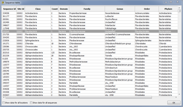
The Sequence Table Viewer plugin display a table indicating the metadata associated with each sequence. Other plugins and custom Python scripts can be used to add data to the Sequence Table. By default, only data for active locations and active sequences is shown. To show data for all locations check the Show data for all locations checkbox. To show data for all sequences check the Show data for all sequences checkbox.
Reference Condition Analysis
- Overview:
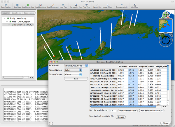
- The Reference Condition Analysis plugin is used to evaluate impacts on biodiversity by computing the expected diversity based on several types of habitat metadata and compares these to the observed diversity.
- Also, see the RCA_Tutorial.
- Requirements:
- R with the Vegan library must be installed on your system (see the GenGIS manual).
- Running RCA:
- Choose the appropriate RCA Model (currently only 'atlantic_rca_model' available). Select the appropriate data labels for Taxon Names and Taxon Counts.
- Browsing Results:
- The O/E (Observed over Expected diversity ratios) are displayed in the table for various alpha diversity measures including Richness, Shannon, Simpson, Pielou, and Berker-Parker.
- Each of these results can be plotted on the main GenGIS map by selecting a column in the table, optionally adjusting the "Bar plot scale factor", and clicking "Plot Selected Data".
- The data can be exported from the plugin table into GenGIS as another metadata habitat field allowing the use of other plugins (e.g. Linear Regression) by selecting a column and clicking "Add Selected To GenGIS".
- Lastly, the entire table of results can be saved to a tab-delimited file by using the "Browse" button.
Show Spread
The Show Spread plugin allows subsets of location and sequence data to be visualized by stepping through any data field, either cumulatively or subset-by-subset. The user is required to provide a base map and location file as a minimum. Show Spread can also add branches to a geophylogeny as entities appear (and disappear).
Default Components
Data: The data field to be iterated over by Show Spread. Only activated location fields will be used.
Sort: Visualize data in descending or ascending order.
Start: The starting point for the iteration.
Stop: The stopping point for the iteration.
Number of Steps: The number of divisions to be made in the data between the start and stop points.
Time per Step: The length of each step in tenths of a second.
OK: Run Show Spread.
Close: Close Show Spread.
?: Access the Help page for Show Spread.
Advanced Components
Colour by Intensity: Recolour locations based on the number of sequences displayed.
Binning: Display individual bins rather than cumulative data. Bin size will have to be defined.
Step Size: The size of a step taken by each increment of Show Spread.
Bin Start: The lower boundary (distance) for data to be considered inside a discrete bin.
Bin End: The upper boundary (distance) for data to be considered inside a discrete bin.
D/M/Y vs. M/D/Y: Whether dates used to define bins are to be interpreted as Day/Month/Year or Month/Day/Year.
Restore: Restores the size and colour of locations to their state previous to running Show Spread.
