Body Location Tutorial

Introduction

GenGIS is a free and open-source bioinformatics application that allows geographic data to be merged with information about biological sequences collected from the environment. It consists of a 3D graphical user interface in which the user can navigate and explore the data, as well as a Python interface that allows easy scripting of statistical analyses using the Rpy libraries.

In this tutorial, we examine samples collected from a set of 28 distinct body sites (Costello et al., 2009) in order to profile the taxonomic composition and diversity of the sampled sequences. Although the original paper had multiple subjects who were sampled over time, here we pool the data for simplicity's sake. This tutorial demonstrates the use of the Rpy statistical libraries and some of the bundled plugins. To follow along with this tutorial download the data:

• Costello data set

Loading Data

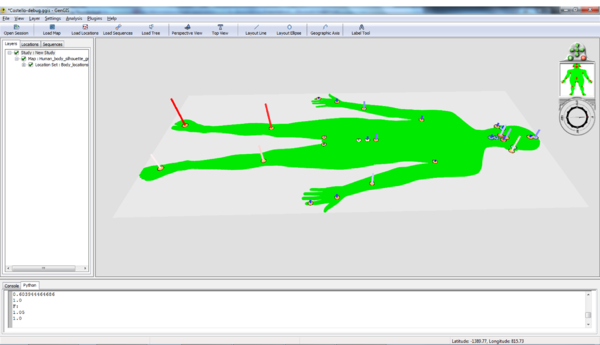
The body site data consist of a .jpeg silhouette of the human body (Human_body_silhouette_green.jpg), originally sourced from (Wikimedia Commons), location data (Body_locations_All.csv) based on the mapping of particular body locations to pixels in the image, and sequence data (CostSequencesRDP_ten.csv). In order to speed things up a bit, the sequence file has been downsampled 10x at random. There is also a Python script that runs a set of R commands and generates heatmaps (Heatmap.py). Load these data files into GenGIS. For basic information on using the GenGIS interface and loading data please see the Banza Katydid Tutorial.

If the default green body / orange locations is not your style, see [[GOS_Tutorial | GOS Tutorial] to change the location colour scheme. Colouring by type will distinguish between skin, gut, etc. locations.

Using the Plugins

Plugins in GenGIS offer the ability to perform frequently used procedures with the help of a graphical user interface. The main release of GenGIS has several plugins, and users can develop others using the Python language, optionally Rpy2 and Numpy, and GenGIS functions that are exposed to Python. Here we show how to use two of the default plugins.

Calculating alpha diversity

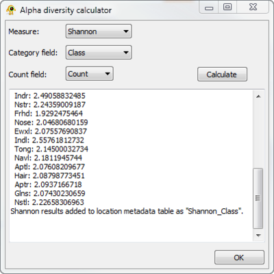
The sequence file contains taxonomic information at the ranks of phylum and class, so we can calculate several sitewise measures of diversity using the Alpha diversity plugin. Open "Alpha diversity" from the "Plugins" menu, and select "Shannon" as the measure. We will keep the default categogy (class). Click the "Calculate" button to generate the results below:

Figure 1. Alpha diversity plugin window.

Linear regression

The regression plugin allows linear regression using data from the sequence and the location files. This allows us to test hypotheses about the relationship between two environmental variables, between an environmental variable and a sequence-based attribute, or between two sequence attributes. As an example, we can test for a relationship between the relative abundance of class Clostridia in different samples, and the overall diversity of that sample. Since Clostridia contains known pathogens (although not exclusively since many gut commensals are found in this group), we might expect that communities enriched in Clostridia have lower diversity overall.

Open "Linear regression" from the "Plugins" menu, and under "Independent Data" select "Use Sequence Data". After a brief pause, the independent variable will default to "Class". From the "Independent Subtype" drop-down menu, choose "Clostridia". For the "Dependent variable (y)", choose the class-based Shannon measure we computed above. Now click the Calculate button, and after a brief pause the following results should appear:

Figure 2. Linear regression plugin window.

The results of the analysis are shown in the lower left-hand corner, and the plot shows, if anything, a weak positive trend with an unimpressive p-value. Two sites appear to be enriched in Clostridia relative to the others: which ones are they?

Results from this plugin are propagated to this window via the "Viewport Display" options. The default action is to plot regression residuals on the map, but we can change this to show either of the variables we just examined. Select "x data" in the Plot Type drop-down menu, and click Calculate again. The regression doesn't change, but now we can switch over to the map window to see the association of Clostridium frequencies with different body sites. The highest frequencies in this pincushion example are seen in the knees and the feet, although the right ear is also somewhat enriched in Clostridia, possibly due to a very high frequency in one of the right ear samples that is summarized here.

Figure 3. Clostridium frequencies plotted on the human body sites.

The Mantel test plugin is structured in a very similar way to the linear regression plugin, but it operates on pairwise distances between sites rather than directly on the values associated with the sites. The exact same procedure can be followed as above, with the additional opportunity to include geographic distances (which are undefined in this case) or Euclidean distances between sites as a variable. The Mantel test is widely used in ecological studies, see for instance Hughes Martiny et al. (2006).

Running R commands directly in the Python console

The inclusion of the (http://rpy.sourceforge.net/rpy2.html Rpy2 libraries) allows R commands to be embedded in a Python script. This allows you to perform statistical analyses interactively in the Python console, and to create external scripts that can be invoked with a single command to the console.

A longer Rpy2 script

If we want to do fancier things using R, then it makes sense to write a script and execute that script within the GenGIS console. Here is an example of how to generate heatmaps of your data using a Python script. The example here is the creatively named "heatmap.py".

First, you need to tell the GenGIS Python interpreter where to find the script. If the script is not in one of the default locations, here is one way to help GenGIS find it:

sys.path.append("C:\\Projects\\GenGIS\\v2.0-devel\\Costello-tutorial")

Then any files in the Windows folder "C:\Projects\GenGIS\v2.0-devel\Costello-tutorial" will be visible to GenGIS. Next, we need to bring Heatmap into scope:

import Heatmap

Now, for the script itself. The objective is to allow the user to specify a column from the sequence file, and a list of two or more labels from that column, which will generate the raw data to be displayed in the heatmap. The contents of the script are explained below.

First, we import the critical libraries:

import GenGIS
import rpy2
import rpy2.robjects as robjects

Then declare the subroutine. Our first action will be to shorten 'robjects.r' to 'r', in order to simplify the syntax of R function calls.

### RunHeatmap generates a heatmap representation of the relative frequency of different sequence file attributes across all locations.
### Two parameters must be passed:
###    columnnToUse: a column heading from the sequence file
###    labelsToUse: a list object containing at least two different labels from the selected column.
###
### Example usage: Heatmap.RunHeatmap("Phylum",["Bacteroides","Firmicutes"])

def RunHeatmap(columnToUse,labelsToUse):
	
	r = robjects.r

We next want to identify the GenGIS layers for each location. We save a list of these as 'locs' by executing the API call:

	### Identify all active location layers
	locs = GenGIS.layerTree.GetLocationSetLayer(0).GetAllActiveLocationLayers()

We will now loop over each layer in turn, counting up both the number of labels of each requested type (i.e., that were passed as the second argument to RunHeatmap) and the total number of sequences associated with each location. The latter count is needed to normalize the counts of interest.

	### Dictionary of sequence counts by location for each of the requested labels
	seqCounts = {}
	
	### Dictionary of total sequence counts by location for normalization
	allCounts = {}
	
	### Iterate through the sequence data and build the dictionary of frequencies
	for loc in locs:
	
		seqCounts[loc] = {}
		allCounts[loc] = 0
		for addLabel in labelsToUse:
			seqCounts[loc][addLabel] = 0
	
		### Some sequences may be disabled, ignore them
		seqLayers = loc.GetAllActiveSequenceLayers()
		sc = len(seqLayers)
		allCounts[loc] = sc
	
		for j in xrange(0, sc):
				data = seqLayers[j].GetController().GetData()
				thisLabel = data[columnToUse]
				if thisLabel in labelsToUse:
					seqCounts[loc][thisLabel] += 1

A couple of important things are going on here: first, we initialize the counts of all interesting labels to zero. The call to loc.GetAllActiveSequenceLayers() returns a list of all sequences associated with the current site. We then iterate through each sequence, incrementing the global count, AND the specific count if it has one of the labels we're looking for.

The astute reader will notice that we haven't done anything with Rpy2 yet, but that is about to change. To plot a sensible heatmap we need three items: the data matrix, and the labels for the rows and columns. Let's build those label lists now:

	numLocs = len(locs)
	numLabels = len(labelsToUse)
		
	### The column and row labels
	yVec = r["c"](robjects.StrVector(labelsToUse))
	xVec = r["c"](robjects.StrVector([locX.GetController().GetData()["Organ"] for locX in locs]))

This is a good opportunity to emphasize the syntax differences between Rpy2 version 2.03 (the version used by GenGIS) and versions 2.1 and higher. These lists are built differently, and the example above is based on the [Version 2.08 documentation].

The row and column labels must be string vectors invoked using R's c(1, 2, 3, ...) syntax: the above rpy2 calls are equivalent to this. The Python list comprehension in 'xVec' collects the value of the "Organ" column from the Location object. This corresponds to the appropriate column in the location file.

Now, let's build the normalized data matrix:

	### Now build the R matrix
	preList = []
	for i in xrange(0,numLocs):
		for j in xrange(0,numLabels):
			preList.append(seqCounts[locs[i]][labelsToUse[j]] / float(allCounts[locs[i]]))

	comVec = r["c"](robjects.FloatVector(preList))
	m = r.matrix(comVec, nrow = numLocs, byrow = True)

The first part is plain old Python. We then need to create an R floating-point vector, and push that into a matrix with the appropriate number of rows (28).

To prepare for the heatmap function call, we pass our matrix 'm', and our label vectors 'xVec' and 'yVec' into the global scope of the R environment. This way future R function calls will be able to see them.

	robjects.globalEnv["m"] = m
	robjects.globalEnv["xVec"] = xVec
	robjects.globalEnv["yVec"] = yVec

And now we're finally ready to generate the heatmap. The options to the heatmap function can be found in the R documentation.

	### And finally, the heatmap
	r("heatmap(m, col = topo.colors(100), scale='none', labCol=yVec, labRow=xVec, margins=c(10,10),cexCol=1.4)")

As an example of usage, invoking RunHeatmap with the following command:

Heatmap.RunHeatmap("Phylum",["Bacteroidetes","Firmicutes","Proteobacteria"])

should produce the following image.

Figure 4. Heatmap showing the distribution of three phyla across 28 different body sites.

Contact Information

We encourage you to send us suggestions for new features. GenGIS is in active development and we are interested in discussing all potential applications of this software. Suggestions, comments, and bug reports can be sent to Rob Beiko (beiko@cs.dal.ca). If reporting a bug, please provide as much information as possible and, if possible, a simplified version of the data set which causes the bug. This will allow us to quickly resolve the issue.

References

Costello EK, Lauber CL, Hamady M, Fierer N, Gordon JI, Knight R. 2009. Bacterial community variation in human body habitats across space and time. Science, 326: 1694-1697. (Abstract)

Martiny JB, Bohannan BJ, Brown JH, Colwell RK, Fuhrman JA, Green JL, Horner-Devine MC, Kane M, Krumins JA, Kuske CR, Morin PJ, Naeem S, Ovreås L, Reysenbach AL, Smith VH, Staley JT. 2006. Microbial biogeography: putting microorganisms on the map. Nature Review Microbiology, 4: 102-112. (Abstract)

Parks DH, Porter M, Churcher S, Wang S, Blouin C, Whalley J, Brooks S and Beiko RG. 2009. GenGIS: A geospatial information system for genomic data. Genome Research, 19: 1896-1904. (Abstract)