Katydid Tutorial
Contents
Introduction
GenGIS is a free and open-source bioinformatics application that allows geographic data to be merged with information about biological sequences collected from the environment. It consists of a 3D graphical user interface in which the user can navigate and explore the data, as well as a Python interface that allows easy scripting of statistical analyses using the Rpy libraries.
In this tutorial, we consider the phylogenetic tree of Banza katydids (acoustic insects) from the Hawaiian Islands recently recovered by Shapiro et al., 2006. GenGIS will be used to investigate whether or not this phylogeny is related to the geography of the Hawaiian Islands. A video walkthrough of this tutorial is also available on the GenGIS website. To follow along with this tutorial download the data:
Overview of User Interface
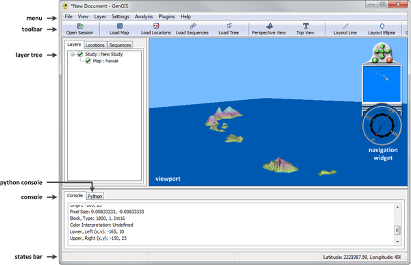
The graphical user interface for GenGIS consists of a collection of different interface elements (Fig. 1). All features of GenGIS can be access through the Menu. The most commonly used features are exposed on the Toolbar. Data loaded into GenGIS is organized into a Layer Tree, which is made explicit to the user in the panel on the left. This hierarchical structure provides a natural organization of data and allows the properties of related data items to be set easily. Data visualizations are displayed in the 3D Viewport. Mouse navigation within this 3D environment follows a standard world-in-hand navigation model. Alternatively, the camera position and angle can be modified using the Navigation Widget, which also provides an overview map. Almost all features available through the graphical user interface can be accessed within the Python Console window. This includes loading data layers, modifying camera parameters, and accessing location or sequence data. Information about interface elements or graphical features within the Viewport is displayed on the Statusbar.
Loading Data
Data can be loaded through the Layer menu or the toolbar (Fig. 2). The ordering of menu items and toolbar buttons correspond to the order in which data should typically be loaded.
Load the map hawaii.ascii using the Add map toolbar button. This will bring up a progress dialog indicating that the map is being loaded. Once the map is finished loading it appears in the Layer Tree panel.
- Mouse Navigation: You can move the map by holding down the left mouse button while moving the mouse. To change the pitch of the camera, hold the right mouse button down and move the mouse up and down. Similarly, to rotate the map move the mouse left or right while holding down the right mouse button. The camera can be zoomed using the scroll wheel on your mouse.
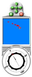
- Navigation Widget: The navigation widget can also be used to navigate around the map (Fig. 3). The arrows at the top allow the map to be moved and the plus and minus button let one zoom in and out of the map. Clicking on the compass and dragging the mouse around the compass face allows one to rotate the map. User can jump to a specific point in the map by clicking within the overview map.
- Predefined Views: GenGIS also provides two convenient default views. To quickly switch to a perspective view or a top down view use either the View→Camera Position menu items or the corresponding toolbar buttons (Fig. 4).
Loading a Location Set
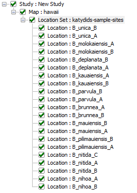
A map can have any number of location sets associated with it. Load the location set (sample sites) in katydids-sample-sites.csv by first selecting the map layer in the Layer Tree and then clicking the Add location set toolbar button. Once the location set is finished loading it appears in the Layer Tree panel. By default, the locations appear as orange circles within the Viewport. Expanding the location set layer shows all locations contained within the set (Fig. 5). Individual locations or an entire location set can be hidden by checking or unchecking the layer. All elements below a given layer can be hidden from view by unchecking the layer.
Loading a Tree
Multiple geographic tree models can be associated with a single map. Load the Katydid phylogeny in katydids-ML-tree.gtm by first selecting the map layer in the Layer Tree and then clicking the Add tree toolbar button. By default, the tree will appear as a 3D geophylogeny. By navigating around this geophylogeny one can qualitatively investigate whether or not the geography of the Hawaiian Islands appears to have played an important role in the phylogenetic relationships between Katydid species.
Changing Visual Properties
GenGIS gives users considerable control over the visual properties of the data visualizations in the Viewport. This allows different aspects of the data to be emphasized which facilitates the exploration and communication of different hypotheses.
Map Properties
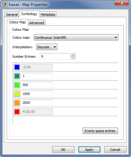
To modify the visual properties of the map, right-click on the map layer in the Layer Tree and select Properties from the pop-up menu. This will bring up the Map Properties Dialog Box (Fig. 6). This dialog box consists of three sections or tabs. On the General tab, the name of the map can be changed and general information about the layer is provided. The Metadata tab indicates specific properties of the map such as its dimensions and geographical extents. Visual properties of the map can be set in the Symbology tab. The Colour Map sub-tab allows users to specify how colours are mapped to elevation. Modify the properties on this page so they reflect those given in Figure 6 and then hit the Apply button. This will update the map with the new colour map. Under the Advanced sub-tab, set the Vertical Exaggeration to 10 and hit Apply. This scales the elevation of each point in the map which can be useful for visualizing differences in elevation. Click OK to exit the property dialog.
Location Set Properties
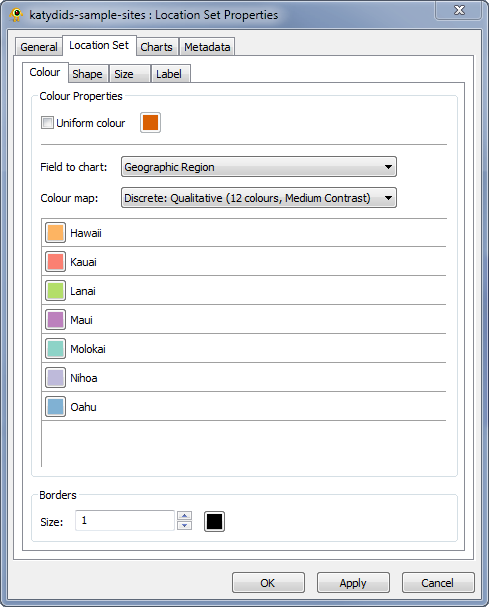
Properties common to all locations can be set through the Location Set Properties Dialog Box (Fig. 7). To open this dialog box, right-clicking the Location Set layer in the Layer Tree and select Properties from the pop-up menu. The General and Metadata tab contain useful information about this layer. On the Chart tab, pie charts can be configured to indicate different properties of any sequence data associated with the location sites. Here we will change the appearance of the location sites in order to emphasize which major geographic areas (e.g., Hawaii, East Maui, Lanai) each sample site belongs to. Later we will modify the appearance of our geophylogeny such that this colouring allows us to better understand how geography has influenced the evolutionary history of Banza katydids. To set the colour of locations based on their geographic area first uncheck the Uniform colour checkbox and then change the Field to chart to Geographic Region. Now change the colour map to Discrete: Qualitative (12 colours, Medium Contrast) as shown in Figure 7 and hit OK. Note that any field specified in the katydids-sample-sites.csv can be used to set the colour, shape, and size of the location set markers. This allows different aspects of the data to be simultaneously visualized.
Tree Properties
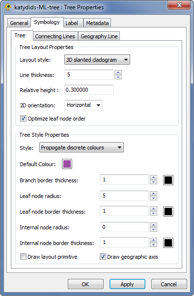
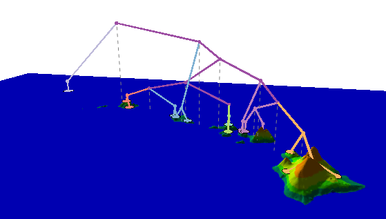
To modify the visual properties of the tree, right-click on the tree layer in the Layer Tree and select Properties from the pop-up menu. This will bring up the Tree Properties Dialog Box (Fig. 8). The visual properties of labels for the leaf nodes of a tree can be modified in the Labels tab. Visual properties of the tree are set in the Symbology tab. We will discuss many of these properties in the next section, but for now change the Line thickness to 5, the Relative height of the tree to 0.3, the tree Style to Propogate discrete colours, and the Internal node radius to zero as shown in Figure 8. Click Apply when done and observe how the colours of branches in the tree now correlate with the location colours (Fig. 9). Colours are propagate up from the leaf nodes of the tree until the children of a node have different colours, at which point the default colour will be used for all branches above this node.
Your Viewport should now be similar to Figure 9. Assigning colours to locations based on their geographic region emphasizes the role of geography on the evolution of Banza katydids. As an exercise, try colouring the locations based on Species. This produces a similar tree, but places more emphases on the position of different species in the tree.
Quantitative Analysis of Geographic Structure
The 3D geophylogeny illustrated in Figure 9 provides strong qualitative evidence that geography has had a substantial influence on the evolution of Banza katydids. GenGIS also allows a quantitative analysis of the role of geography to be performed. This is done by drawing a 2D geophylogeny where the leaf nodes are ordered such that they maximize the goodness-of-fit between the tree and geography (Parks and Beiko, 2009; Parks et al., 2009). To perform this analysis follow these steps:
- Switch to a top view by clicking on the Top view toolbar button (Fig. 4).
- Click on the Layout line toolbar button (Fig. 10).
- Draw a layout line as shown in Figure 11A. The tree will be drawn on the right-hand side of this line as you ‘walk’ from the starting point of the line to the end point of the line. Since we want the tree to appear below the island chain, the line should be drawn from left to right. Don’t worry if you draw it backwards as it can easily be moved.
- Right-click on the tree layer in the Layer Tree and select 2D cladogram from the pop-up menu. This causes a 2D geophylogeny to be drawn as shown in Figure 11B. Any crossings that occur between the two dashed lines in this figure indicate discordance between the phylogenetic tree and geography. The presence of relatively few crossings provides strong evidence that geography played an important role in shaping the relationships expressed by the phylogenetic tree.
- Try clicking on different nodes within the geophylogeny and the geographic locations. These elements can be selected (highlighted) in order to explore and emphasize different aspects of the data.
- At this point, you may wish to try changing some of the properties in the Tree Properties Dialog Box to see what effect they have on the 2D geophylogeny.
- Click on the root node of the geophylogeny. Notice that the second panel of the Statusbar indicates that below this node there are eight crossings. To test if this is statistically significant, a random permutation test can be performed (Parks and Beiko, 2009). Right-click on the root node, and select Perform significance test on subtree from the pop-up menu. A dialog box will appear indicating the test is being performed. The results will be reported in the Console window. You should get a p-value near 0.001 indicating that the number of observed crossings is significantly smaller than would be expected by chance alone.

Going Further
This tutorial does not describe all the functionality of GenGIS. For further information, please see one of our other tutorials, the manual, or start exploring GenGIS for yourself. Below are a few interesting features not discussed in this tutorial.
Pie Charts
Sequence data was not considered in this tutorial. GenGIS provides functionality for loading, analyzing, and visualizing sequence data. Using the Python Console different phylogenetic and statistical techniques can be applied to sequence data. Summaries of metadata associated with sequences can be directly visualized in the Viewport as a set of pie charts.
Making Movies
With minimal effort, fly-through videos can be constructed to help illustrate important aspects of the data. See the GenGIS manual for details on how to modify the camera position through the Python console. A collection of useful functions for creating movies is available in the movieHelper.py file in the scripts directory. Example movies made with GenGIS can be found on our website and details on using the movieHelper.py script is provided in the GenGIS Manual.
Contact Information
We encourage you to send us suggestions for new features. GenGIS is in active development and we are interested in discussing all potential applications of this software. Suggestions, comments, and bug reports can be sent to Rob Beiko (beiko@cs.dal.ca). If reporting a bug, please provide as much information as possible and, if possible, a simplified version of the data set which causes the bug. This will allow us to quickly resolve the issue.
References
Parks DH and Beiko RG. 2009. Quantitative Visualizations of Hierarchically Organized Data in a Geographic Context. 27th International Conference on Geoinformatics, Fairfax, Virgina. IEEE Xplore
Parks DH, Porter M, Churcher S, Wang S, Blouin C, Whalley J, Brooks S and Beiko RG. 2009. GenGIS: A geospatial information system for genomic data. Genome Research, 19: 1896-1904.
Shapiro LH, Strazanac JS, and Roderick GK. 2006. Molecular phylogeny of Banza (Orthoptera: Tettigoniidae), the endemic katydids of the Hawaiian Archipelago. Mol. Phylogenet. Evol. 41:53-63. Pubmed
