The GenGIS 2.5 Manual
Welcome to the GenGIS 2.5 manual. The sections below provide enough information to configure and start using GenGIS. Stay tuned for updates and send us your feedback when you get an opportunity.
Contents
Introduction / Overview of GenGIS
Purpose
Geography has always been an important component of evolutionary and ecological theory. The advent of sequence typing approaches such as 16S ribotyping, DNA barcoding using the COX1 gene, and multi-locus sequence typing, gives us the opportunity to understand how communities of organisms interact, disperse and evolve. This sequencing revolution is tightly coupled to the development of new algorithms for assessing and comparing populations based on their genes.
Coupled with these developments is the availability of high quality, public domain digital map data. By integrating molecular data with cartography and habitat parameters, we can visualize the geographic and ecological factors that influence community composition and function.
GenGIS is designed to bring these components together into a single software package that satisfies the following criteria:
- Free and Open Source
- GenGIS is released under a Creative Commons Attribution - Share Alike 3.0 license, and we have made extensive use of other free packages such as wxWidgets, R, and Python. Making GenGIS freely available allows it to be downloaded and used anywhere in the world, and allows users to inspect and modify the source code.
- User-Friendly Interface
- Although GenGIS is built to deal with challenging scientific questions, our goal is to make the software easy to use. This is particularly important as many users will have little experience with digital map data, apart from applications such as Google Earth.
- Adaptible and Extensible
- The principal strength of many open-source projects lies in the ability of a loosely organized community of users to develop and enhance the software: R and BioPerl are two examples of successful open-source projects with many contributors. Since the potential applications of GenGIS are much broader than those we have in mind, we aim to make it as easy as possible to extend its capabilities by exposing the internal data structures and offering a plugin architecture.
Citing GenGIS
The best citation for GenGIS is indicated in boldface on the Main GenGIS page.
Where to go for Help
- The latest version of the GenGIS manual.
- The current master list of plugins, with documentation, is available at the Plugin Description page.
- Text and video tutorials are available on the Tutorials page.
- The FAQ page keeps track of GenGIS-related questions.
- Please email with any questions or feedback about the software.
Installation
Getting the Latest Version of GenGIS
Download the latest version for Windows or Mac to get started visualizing and analyzing data in GenGIS.
System Requirements
GenGIS has been developed and tested on the following operating systems:
- Windows (XP, Vista & 7) 32-bit binaries compatible with 64-bit Windows releases.
- Windows XP requires the Microsoft Visual C++ 2008 SP1 Redistributable Package (x86).
- Mac OS X (v10.5 'Leopard', v10.6 'Snow Leopard' and v10.7 'Lion') Intel-based only.
Developer Version – building from source code
|
The source code for GenGIS is available on the Download page. | |
| Building on Windows | GenGIS can be compiled using Microsoft Visual C++ 2008 Express Edition. The Visual Studio solution file (GenGIS.sln) is located in the 'win32/build/msvc' directory. Please note that the built-in Python console is only available in Release builds. |
|---|---|
| Building on MacOSX | GenGIS can be compiled using the Makefile located in the 'mac/build/gcc' directory. To compile, simply run 'make' within a terminal. Development has been performed using the gcc 4.3.3 compiler. |
R and GenGIS
GenGIS integrates with the R programming language to provide additional statistics and visualization tools. Calls to the R environment are made by certain GenGIS plugins (e.g., Mantel).
To configure R with GenGIS:
- Download and install R (make sure to close GenGIS during the R installation).
- Windows: For Windows users, run the R Auto-Configuration Utility from the GenGIS Settings menu.
- Mac: No additional configuration is required on Mac systems.
Manually Configuring R (Windows)
Note: the R Auto-Configuration Utility performs these configurations automatically.
Recent versions of R (e.g., v2.14.1) use a different installation file structure that is incompatible with the Windows version of GenGIS. The issue can be resolved by means of a harmless workaround described below. If running GenGIS on MacOSX, you may skip this section. For Windows XP users, the path to the R bin directory (e.g., C:\Program Files\R\R-2.14.1\bin) needs to be set within the Windows PATH environment variable.
Manually Transferring DLLs:
| Windows XP, Vista & 7 |
|
|---|
Manually Setting the PATH Variable:
| Windows XP Only |
|
|---|
R Auto-Configuration Utility
The R Auto-Configuration Utility configures R to work with GenGIS and is located in the Settings menu.
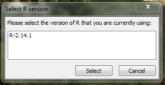
- For recent versions of R (e.g., 2.14.1), a GenGIS dialog will appear prompting to select the latest version of R being used on the system:
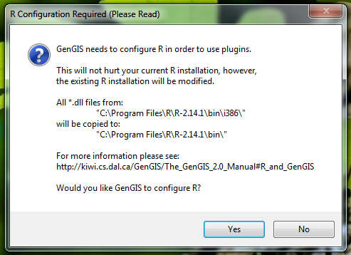
- After the selection, a confirmation window will appear:
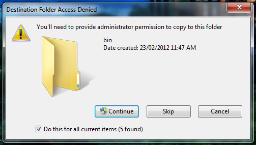
- On Windows Vista/7, you will need to provide the Windows User Account Control (UAC) permission to complete the configuration:
- On Windows Vista/7, R should now work without requiring a restart of GenGIS.
- Windows XP users will be prompted to add the R installation directory to the Windows Path variable. After completing this step a reboot of Windows is required for the changes to take effect.
Input data
Data File Types
GenGIS works with four different types of data files:
Data files should be loaded in the following orders:
Map(s) → Location → Sequence → Tree
or
Map(s) → Location → Tree
Version 2.1 and above: GenGIS now supports vector data, with or without an underlying raster. If a raster file is to be used, it should be loaded before any vector data. If no raster is provided, the first vector file loaded will be used to initialize the map environment, and will be listed first. The minimap boundaries and default views will be based on the dimensions of this vector, even if other vector files are added and the original vector subsequently deleted. Any number of vector files can be loaded and viewed in GenGIS; these can be added and deleted at any stage.
GenGIS currently supports a single location and sequence file during a session. Any number of tree files can be opened.
Note: The location of sequences (sequence file) and leaves (tree file) must each map to an existing location given by the location file. The leaves of a tree file can be identifiers for either locations or sequences.
Maps
GenGIS relies on the Geospatial Data Abstraction Library (GDAL) to import several digital map file formats and projections. More information, including community support and downloads, can be found at the GDAL website.
Note: The 'gdal_merge.py' script, 'gdalwarp.exe' and 'gdal_translate.exe' executables have been very useful in preparing maps compatible with GenGIS.
Supported raster formats
GenGIS supports the formats listed on the GDAL Raster Formats page. Note that not all formats have been tested at this time. The following formats have been found to work reliably:
- GeoTIFF
- Arc/Info ASCIIGRID
- USGS DEM (and variations thereof)
Supported vector formats
We have tested GenGIS on a number of different ESRI shape files (typically ending in .shp).
Projections
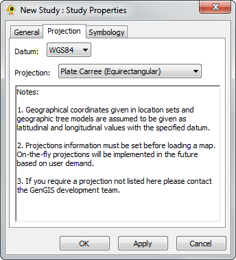
If you wish to use a specific projection, you must specify it before loading your map - GenGIS is unable to render reprojections on the fly. This is particularly true if you are loading the default world map (from GTOPO30) that ships with GenGIS: the default Mercator projection stretches the polar regions, whereas Plate Carre or Robinson will provide a much less distorted world view.
To specify the projection before loading the map, right click "New Study : Study" in the Layers tab, and select Properties. Selecting the Projection tab will allow you to choose your projection.
GenGIS currently does not support projections in which a single point is displayed in multiple locations. The best example of this is the default world map, which is modified to stretch from 89.9 degrees North to 89.9 degrees South latitude. Since the poles stretch across the entire upper and lower edges of a map in a projection such as Plate Carre, GenGIS is unable to display these properly.
Warning: Currently the projections are not working properly. You might get errors in some cases.
Typical limits on map size
Higher processor speeds and more system RAM are required to work effectively with larger maps. Typically one gigabyte of RAM permits working with maps that are 10 megabytes or slightly greater in size.
Reducing Map Size
If the map resolution of is too high for the system hardware being used, the GDAL Utilities 'gdalwarp' or 'gdal_translate' can be used to reduce the density of points in the map. Decreasing the level of detail is an acceptable tradeoff in many cases.
Location File
The location file must be provided in either tab-delimited or comma-separated formats (e.g., the .CSV files that can be exported from Microsoft Excel). The first line of the file must be a series of headers. Each subsequent line should contain a set of attributes for a single location.
- The first entry of the header must be a unique location identifier with the label Site ID or Sample ID.
- A vertical coordinate labelled as Latitude (decimal degrees) or Northing (Universal Transverse Mercator, UTM) must be included but can be present at any column position after the unique location identifier. Note that positive values = north and negative values = south.
- A horizontal coordinate, labelled as Longitude (decimal degrees) or Easting (Universal Transverse Mercator, UTM) must be included but can be present at any column position after the unique location identifier. Note that Positive values = east and negative values = west.
The first line of the file may look something like the following:
Site ID, Latitude, Longitude
or
Site ID, Northing, Easting
depending on the coordinate system.
GenGIS provides the ability to specify many different custom column headers within the Location file, including longer descriptive site names, environmental parameters, or a time stamp. For instance, a location file header might look like this:
Site ID, Latitude, Longitude, File Size, Environment Type, Geographic Location, Site Name, Country
Each of these values must then be specified for every entity (= row in the file), even if they are called NULL or some other placeholder value.
Sequence File
The basic specification of the sequence file is even simpler, with only two required fields:
- A unique location identifier that is also found in the location file
- A unique sequence identifier
The first line of the file must begin with the following column headings:
Site ID, Sequence ID
Columns containing custom information can be added after the two mandatory headings. Each row of the sequence file must define a value for each of the columns identified in the header line. Note that the 'sequence file' need not contain any molecular sequence data, nor do the entities necessarily need to have a one-to-one correspondence to actual sampled sequences.
A simple sequence file might summarize the taxonomic classification of each sampled sequence:
Site ID, Sequence ID, Best_match, Species, Genus, Family, Order, Class, Phylum, Superkingdom
Multiple identical sequences at a location
A count field may be specified within a Sequence File to indicate the number of times a given sequence is present at a given site. This has the benefit of significantly reducing the size of a Sequence File.
Site Id, Sequence Id, Count, Domain, Phylum, Class, Order, Family, Genus, Species
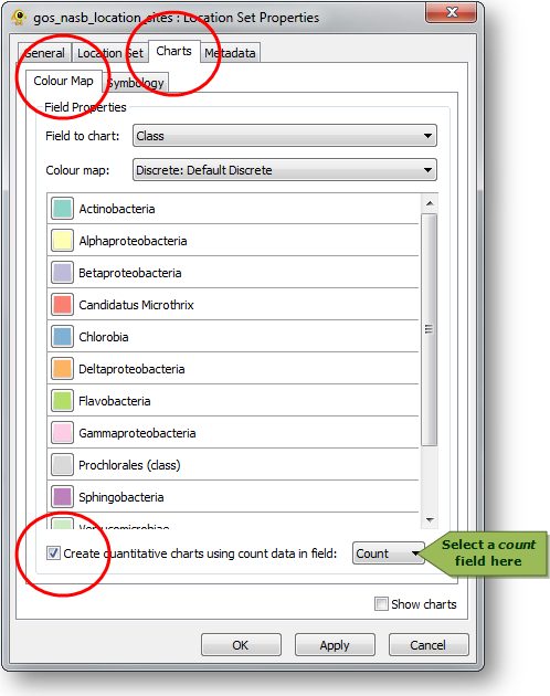
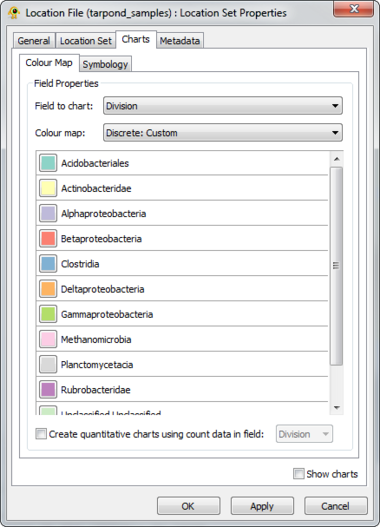
The count field can be assigned any name within the Sequence File. Multiple count fields may be specified indicating different quantitative aspects of a named sequence type such as number of sequences or total base pairs observed. The count field can then be specified in various locations within GenGIS. For example, quantitative pie charts reflecting the number of times each sequence type is observed at a location can be created through the Location Set Properties dialog:
- Open the Location Set Properties dialog
- Navigate to the Charts > Colour Map tab
- Select "Create quantitative charts using count data in field"
- Select the desired count field from the adjacent drop down menu
Tree File
Input trees should adhere to the Newick file format, with the additional constraint that leaf labels must match up exactly with either a Site ID from the location file or a Sequence ID from the sequence file.
The Environment
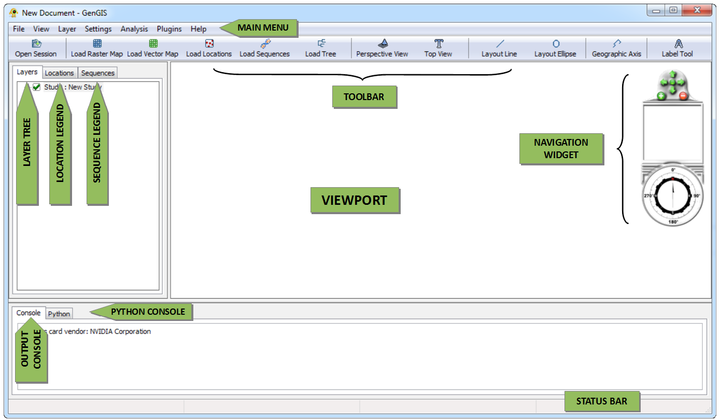
Overview
|
|
|
|
| |
|
|
| |
Menu Items
|
|
Toolbar Buttons
The main toolbar provides easy access to frequently used features.
| Open Session | Open a file to restore a previous GenGIS session. | |
| Add raster map | Add a raster map to the currently selected study. | |
| Add vector map | Add a vector map to the currently selected study. | |
| Add location set | Add a location set to the currently selected map. | |
| Add sequence data | Add sequence data to the currently selected location set. | |
| Add tree | Add a geographic tree model to the currently selected map. | |
| Default perspective view | Move camera to its default perspective position. | |
| Top view | Move camera to give a top-down view of the map. | |
| Draw layout line | Draw a straight line which can be used to layout graphic elements such as a 2D tree or pie charts. | |
| Draw layout ellipse | Draw an ellipse which can be used to layout graphic elements such as a 2D tree or pie charts. | |
| Draw geographic axis | Draw a polyline which can be used to test the goodness-of-fit between a tree and a non-linear geographic axes (see 2D Pylogenetic Trees). |
Note: GenGIS does not support loading multiple maps, location sets or sequence sets. Adding multiple trees is experimental at this time.
GenGIS offers three different options to navigate maps: direct mouse gestures, a navigation widget, and two predefined views.
| Mouse |
| |
|---|---|---|
| Navigation Widget | 
|
|
| Predefined Views | 
|
|
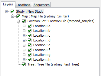
Layer Tree Controller
|
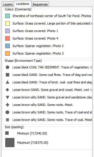
Location Legend
|
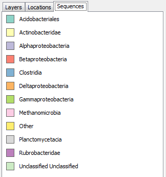
Sequence Legend
|
Console Panels
GenGIS features an output console and a Python console both located at the bottom of the main interface.
Output Console
The Output Console displays a log of successful program operations (e.g., loading data files such as map files) as well as possible errors.
Python Console
The Python console contains a fully-functional Python interpreter that provides access to data structures within GenGIS (e.g., location layer data) and API functions (e.g., the ability to automate camera and lighting controls via Python scripting). The Python console is described in greater detail later in the manual.
Interacting with sample sites
Layer Property Dialogs
Study Layer Properties
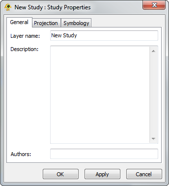
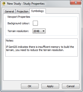
The Study Layer is automatically created during a new session. The Study Properties dialog provides controls to change settings such as study layer metadata (name, description and authors), background colour and terrain resolution. Components of the Study Layer properties dialog are explained in greater detail below.
|
| |||||
|
|
Raster Map Layer Properties
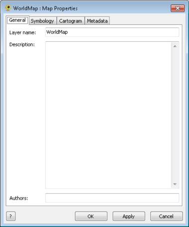
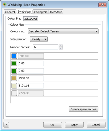
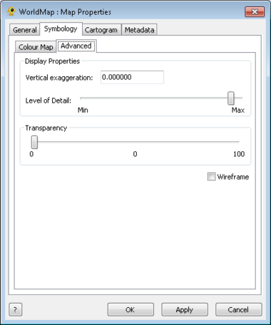
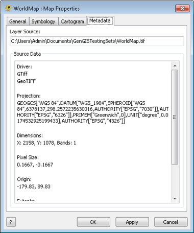
The Raster Map Layer displays a raster map file and directly interacts with other layers (e.g., location, sequence, tree). The Map Layer properties dialog controls settings such as map layer metadata (e.g., name, description), colour scheme and rendering detail. Metadata from the map file (e.g., dimensions, origin) is also displayed. At this time, GenGIS supports a single map layer per session. Components of the Map Layer properties dialog are explained in greater detail below.
|
| ||||
|
| ||||
|
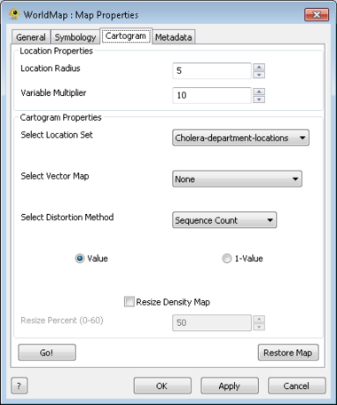
Creating a Cartogram
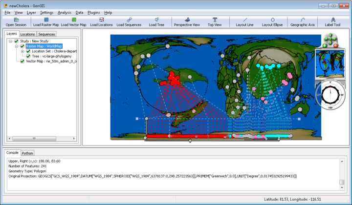
Cartograms are geographic visualization techniques which transfer the distribution of land area in a map from distance to another parameter of interest (such as population). This display technique has been integrated into GenGIS based on the diffusion-based cartogram. To create a cartogram a map and location layer are required. Additional location and vector layers can be transformed with the raster layer. To create a cartogram the Location Radius and Variable Multiplier must be set to some level. Location Radius defines the level of geographic preservation at a regional scale, while Variable Multiplier applies more distortion locally.
Vector Map Layer Properties
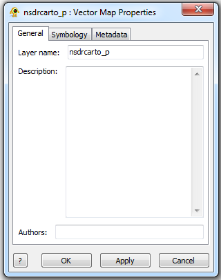
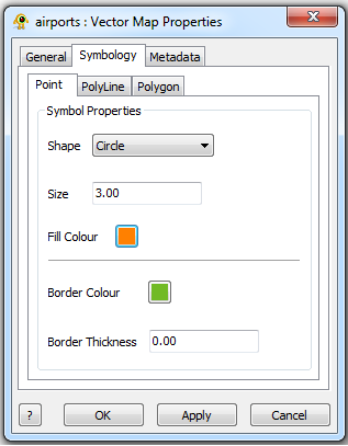
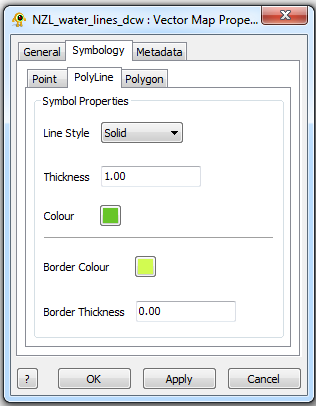
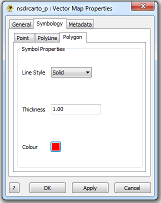
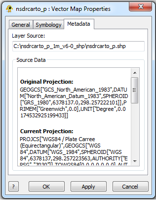
The Vector Map Layer displays a shapefile. One or more than one Shapefiles can be loaded and visuialized in GenGIS. The Vector Map Layer properties dialog controls settings such as vector map layer metadata (e.g., name, description) and visual properties for shapefile features. Metadata for each shapefile (e.g., projection, number of features,...) is also organized and displayed. Components of the Vector Map Layer properties dialog are explained in greater detail below.
|
| ||||
|
| ||||
|
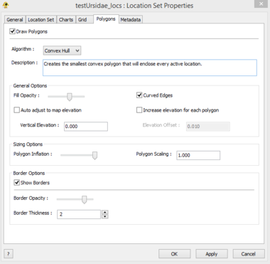
Location Set Layer Properties
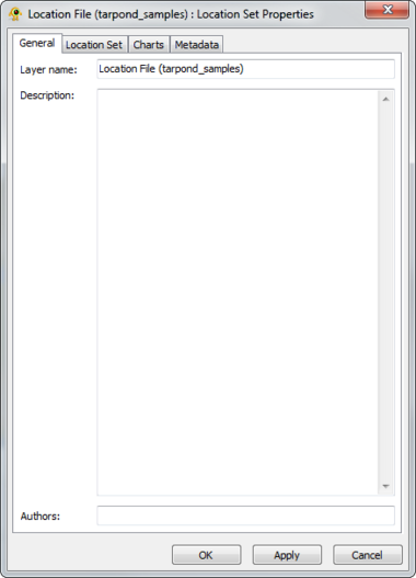
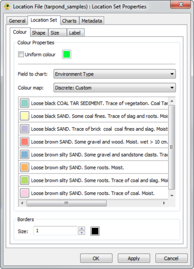
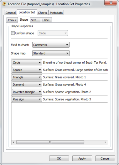
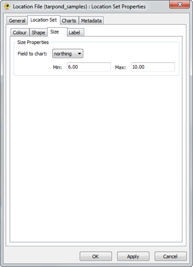
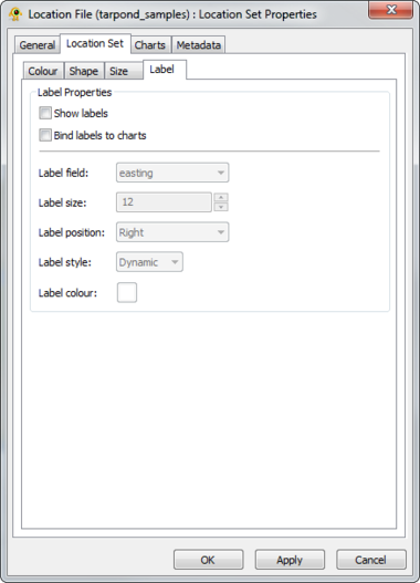
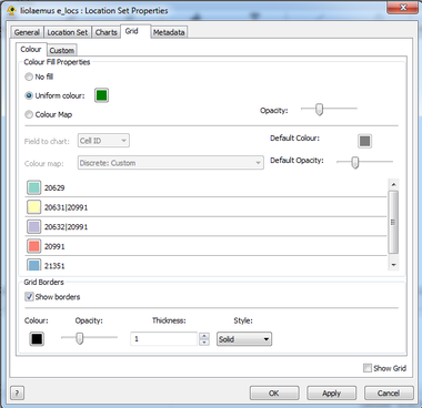
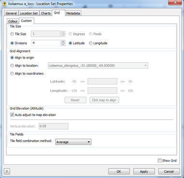
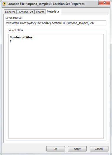
A location file is treated as a location set layer containing several distinct location layers. The Location Set Layer properties dialog controls settings such as location set layer metadata (e.g., name, description) and visual properties for both locations and charts (e.g., colour, size). Metadata from the location file (e.g., number of sites) is also displayed. At this time, GenGIS supports a single location file per session. Components of the Location Set Layer properties dialog are explained in greater detail below.
|
| |||||||
|
| |||||||
|
| |||||||
|
| |||||||
|
| |||||||
|
|
|
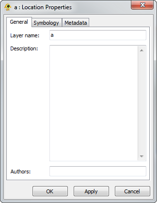
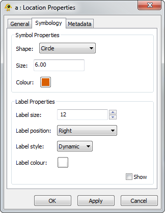
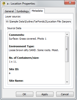
Location Layer Properties
Properties of individual locations are accessible through the Location Layer Properties dialog. Components of the properties dialog are explained in greater detail below.
|
| ||||
|
|
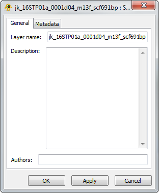
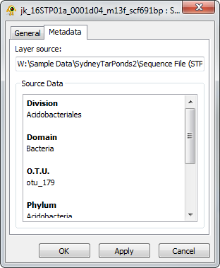
Sequence Layer Properties
The Sequence Properties dialog provides controls to modify sequence layer metadata (e.g., name, description) and also displays sequence file metadata. Components of the Sequence Layer properties dialog are explained in greater detail below.
|
|
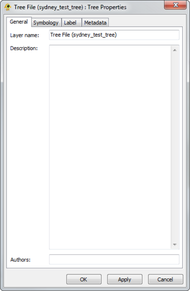
Tree Layer Properties
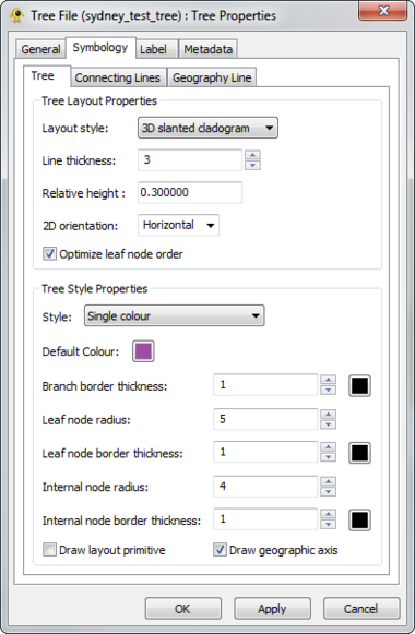
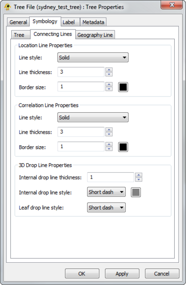
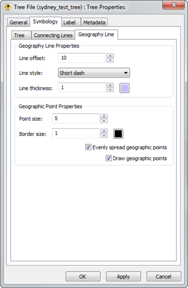
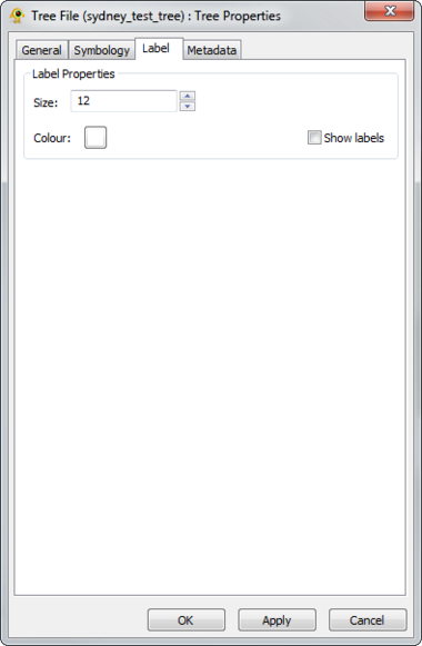
GenGIS supports 2D and 3D trees (e.g., phylogenetic or hierarchical cluster tree). Different display properties (e.g., colour, line width) can be assigned to trees through the Tree Layer Properties dialog. GenGIS supports loading multiple trees during a single session. Components of the Tree Layer properties dialog are explained in greater detail below.
|
| ||||
|
| ||||
|
|
Graphical analysis tools in GenGIS
Basic data visualizations
GenGIS provides a number of ways to visualize data. Chief among these are visualizing summaries of sequence data as charts, and visualizing the relationship between location specific data as 2D or 3D trees. Other visualization are implemented as plugins and custom visualization can be generated through the Python interface.
Visualizing sequence data as charts
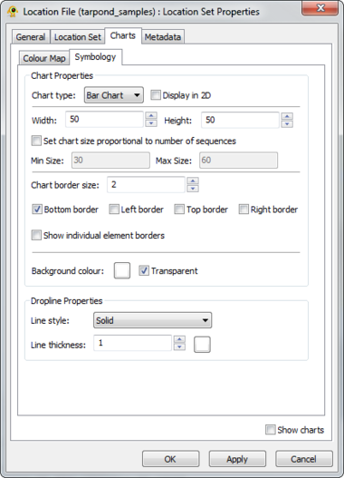
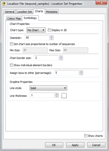
GenGIS supports both bar charts and pie charts to represent sequence data within locations. Charts are configured through Chart tab of the Location Set Layer Properties dialog. The sequence metadata field to graph is set through the Field to chart combobox. The colour assigned to each field element depends on the selected colour map and can be customized as desired. If your Sequence File contains a field indicating the number of times each sequence type was identified at a given location this can be set through the Create quantitative charts using count data in field combobox. By enabling or disabling this feature, qualitative (richness) and quantitative (evenness) pie charts can easily be created. The Symbology tab allows one to specify the type of chart to create and to set properties effecting the appearance of charts. In particular, the size of charts can be set to reflect the number of sequences obtained at a location by enabling the Set chart size proportional to number of sequences checkbox. For pie charts, the abundance at which sequence types (e.g., taxa) are assigned to the Other category is set through the Assign taxa to other field.
|
| |||||
|
|
|
3D Trees
Trees in Newick file format can be loaded into GenGIS. Leaf nodes within a tree must match up with either a Site ID from the location file or a Sequence ID from the sequence file. By default, trees are shown as 3D geophylogenies:
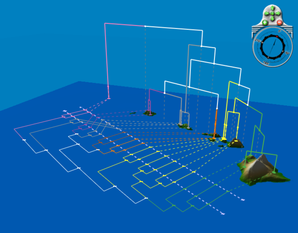
The visual properties of 3D trees are highly customizable and can be modified through the Tree Layer Properties dialog.
2D Trees
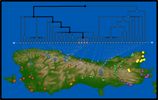
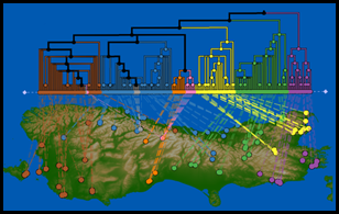
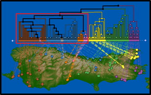
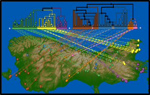
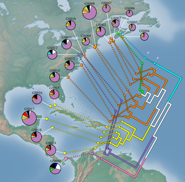
GenGIS supports the quantitative visualization of 2D trees which can be used as an exploratory tool. Specifically, users can define a geographic axis and visualize how well the topology of a tree correlates with the ordering of geographic locations along this axis. This is accomplished by finding the ordering of leaf nodes, subject to the constraints of the tree topology, which minimizes the number of crossings that occur between lines that connect leaf nodes to their associated geographic locations. In this optimal layout, the number of crossings that occur between these lines is a quantitative measure of the amount of discordance which exists between the topology of the tree and the user defined geographic axis. Further information about this quantitative 2D visualization technique can be found in:
- Parks DH and Beiko RG. 2009. Quantitative visualizations of hierarchically organized data in a geographic context. Geoinformatics 2009, Fairfax, VA. (Abstract)
- Parks DH, Porter M, Churcher S, Wang S, Blouin C, Whalley J, Brooks S, and Beiko RG. 2009. GenGIS: A geospatial information system for genomic data. Genome Research, 19: 1896-1904. (Abstract)
Defining axes
To generate a 2D tree, a Layout Line must first be drawn. Select the Layout Line from the main toolbar, click on the map where you would like the line to start, and then click again where you would like the line to end. The 2D tree will always be drawn on the right-hand side of the Layout Line as you walk from the start to the end of the line. To generate a 2D tree, right-click on the Tree Layer in the Layer Tree and select 2D slanted cladogram, 2D cladogram, or 2D phylogram from the pop-up menu.
If you wish to specify a non-linear geographic axes, select Draw geographic axis from the main toolbar. You can now draw a polyline within the Viewport by clicking on the desired start and end points of individual line segments. Press Enter when you are finished drawing the polyline. You can right-click on any polyline vertex and select Extend geographic axis to draw more complicated non-linear axes. Note that only locations which reside close to the specified polyline are considered and all other locations are projected out of the tree.
| Draw layout line | Draw a straight line which can be used to layout graphic elements such as a 2D tree or pie charts. | |
| Draw geographic axis | Draw a polyline which can be used to test the goodness-of-fit between a tree and a non-linear geographic axes (see 2D Pylogenetic Trees). |
Manipulation
The geographic axis being evaluated can be modified dynamically. To modify the geographic axis, simple click on either of the end-points of the Layout Line and drag it to a new location. The vertices defining a non-linear geographic axes can also be modified dynamically. Making the Layout Line shorter will reduce the size of the 2D tree. The height of the tree can also be modified in the Tree Layer Properties dialog. You can also drag the root node of a tree to re-position the tree while keeping the Layout Line at the same orientation.
Zoom into a Sub-tree
Displays the sub-tree defined by the selected node.
|
|
|
Collapse a Sub-tree
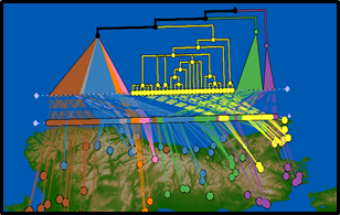
Displays the sub-tree defined by the selected node as a wedge, coloured by the proportional content of all child leaf nodes.
|
|
|
Split a Sub-tree
Removes a sub-tree defined by the highest selected node from the original tree. This node becomes the root node in a new separated tree.
|
|
|
Visual Properties
The visual properties of 2D trees are highly customizable and can be modified through the Tree Layer Properties dialog.
Statistical Test
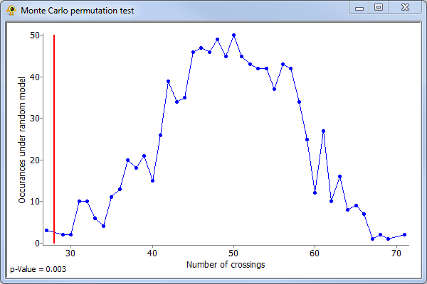
A Monte Carlo permutation test can be used to test whether or not the fit of ordered leaf nodes to geographic points is significantly better than expected by chance alone. This null hypothesis is tested by holding the tree topology, geographic axis, and the association between leaf nodes and geographic locations constant while permuting the ordering of geographic locations along the geographic layout line. After each random permutation, the new optimal ordering of leaf nodes is determined and the number of edge crossings is determined. By generating many random permutations, we obtain an estimate of the probability mass function of the null model. The reported p-value is the fraction of permutations that have a number of crossings fewer than or equal to the number of crossings in the original model. Note: this explanation differs slights from the one given in Parks and Beiko, 2009 where the association between leaf nodes and geographic locations was permuted. In practice, this results in the same null distribution though special care must be taken to properly handle geographic locations which are associated with multiple leaf nodes.
To perform a Monte Carlo permutation test, right-click on the Tree Layer in the Layer Tree and select Perform significant test (on full tree) from the pop-up menu. The permutation test can also be applied to any subtree by right clicking on the root node of the subtree and selecting Perform significant test on subtree from the pop-up menu. The results of the permutation test are shown as a graph which indicates the calculated p-value along with the estimated probability density function. The number of crossings occuring on the actual data is shown by a red line.
Linear Axes Analysis
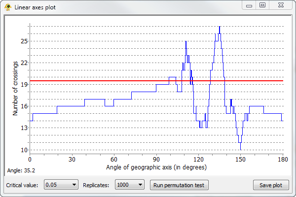
GenGIS allows the number of crossing which occur for all linear gradients to be explored. Right-click on the subtree of the geophylogeny you wish to analyze and select Perform linear axis analysis on subtree. This will produce a graph showing the number of crossings which occur for all possible linear gradients. Clicking on the graph causes the linear layout line to rotate to a given orientation. Running a permutation test causes a red line to be drawn on the plot which indicates the number of crossings at which the specified critical value (i.e., p-value = 0.05) is obtained. That is, linear gradients with orientations resulting in fewer crossings are significant at the selected p-value.
The Python console and API functions
What you can do with the console
The Python Console provides access to a standard Python interpreter. Python is a general-purpose high-level programming language with many packages available for phylogenetics, population genetics, and statistics. Data loaded into GenGIS is exposed to the Python Console allowing quanitative hypothesis testing to be performed directly within GenGIS. Results of analyses can be visualized within the Viewport to aid in interpretation of results and generation of new hypotheses.
Below we give several short examples of using this API. You can also find information about using the API on our tutorials page.
Accessing location site and sequence data
Location site and sequence data can be accessed directly from the Python Console. You can access all location layers using:
locLayers = GenGIS.layerTree.GetLocationSetLayer(0).GetAllLocationLayers()
If you wish to get a list of only the active location layers (i.e., those which are checked), use:
activeLocLayers = GenGIS.layerTree.GetLocationSetLayer(0).GetAllActiveLocationLayers()
Properties of a location are accessed through its controller:
locController = locLayers[0].GetController()
A list of functions supported by the location controller can be obtained with:
dir(locController)
The metadata associated with a location is accessed as a python dictionary:
 metadata = locController.GetData()
 metadata.keys()
 metadata['Site ID']
All sequence layers or all active sequence layers associated with a location layer can be accessed using:
 seqLayers = locLayers[0].GetAllSequenceLayers()
 activeSeqlayers = locLayers[0].GetAllActiveSequenceLayers()
Analogous to location data, data associated with a sequence is accessed through the sequence controller:
 seqController = seqLayers[0].GetController()
 metadata = seqController.GetData()
 metadata.keys()
 metadata['Sequence Id']
Filtering data
We have provided a simple function, filterData, for filtering data. This function is contained in dataHelper.py. As an example, all locations with a temperature greater than 20 can be obtained as follows:
import dataHelper
locLayers = GenGIS.layerTree.GetLocationSetLayer(0).GetAllLocationLayers()
filteredLocLayers = dataHelper.filter(locLayers, 'Temperature', 20, dataHelper.filterFunc.greater)
The function filter takes 4 parameters:
- the data to be filtered
- the field to filter on
- the value to filter on
- a filtering function which returns true for all items passing the filter
Filtering can be done on either strings or numeric values:
import dataHelper
seqLayers = locLayers[0].GetAllSequenceLayers()
filteredSeqLayers = dataHelper.filter(seqLayers, 'Phylum', 'Actinobacteria', dataHelper.filterFunc.equal)
Basic filtering functions are provided in filterFunc.py, but it is easy to write your own filtering functions. For example, the equal filter used above is simply:
def equal(val1, val2):
  return str(val1) == str(val2)
Creating custom data visualizations
Using the VisualLine, VisualMarker, and VisualLabel classes one can create custom data visualizations with GenGIS. The VisualLine class allows user defined lines to be drawn in the Viewport. Suppose we have two locations within our location set with ids of 'GBR' and 'ITA'. We can draw a line between these locations as follows:
# get location layers
locLayers = GenGIS.layerTree.GetLocationSetLayer(0).GetAllLocationLayers()
# create a dictionary indicating the geographic coordinates of each location
locDict = {}
for loc in locLayers:
  locDict[loc.GetController().GetId()] = [loc.GetController().GetLongitude(), loc.GetController().GetLatitude()]

# get the 3D position of GBR and ITA
terrainController = GenGIS.layerTree.GetMapLayer(0).GetController()
gbrPt = GenGIS.Point3D()
terrainController.GeoToGrid(GenGIS.GeoCoord(locDict['GBR'][0], locDict['GBR'][1]), gbrPt)
itaPt = GenGIS.Point3D()
terrainController.GeoToGrid(GenGIS.GeoCoord(locDict['ITA'][0], locDict['ITA'][1]), itaPt)
# draw a solid red line with a width of 2 between these countries
line = GenGIS.VisualLine(GenGIS.Colour(1,0,0), 2, GenGIS.LINE_STYLE.SOLID, GenGIS.Line3D(gbrPt, itaPt))
lineId = GenGIS.graphics.AddLine(line)
GenGIS.viewport.Refresh()
The visual properties of this line can easily be changed at any time to reflect different aspects of your data:
line.SetColour(GenGIS.Colour(0,1,0))
line.SetThickness(5)
line.SetLineStyle(GenGIS.LINE_STYLE.SHORT_DASH)
GenGIS.viewport.Refresh()
We can later remove this line using:
GenGIS.graphics.RemoveLine(lineId)
GenGIS.viewport.Refresh()
The VisualMarker class allows user defined markers to be drawn in the Viewport. It is similar to the VisualLine class. For example, we can draw a blue circle over London which is situated at a longitude 0.128W and a latitude of 51.51N as follows:
# get 3D position of geographic coordinate in Viewport
terrainController = GenGIS.layerTree.GetMapLayer(0).GetController()
pt = GenGIS.Point3D()
terrainController.LatLongToGrid(GenGIS.GeoCoord(-0.128, 51.51), pt)
marker = GenGIS.VisualMarker(GenGIS.Colour(0,0,1), 6, GenGIS.MARKER_SHAPE.CIRCLE, pt)
markerId = GenGIS.graphics.AddMarker(marker)
GenGIS.viewport.Refresh()
VisualLabels can be used to create orthographic (e.g., to indicate a legend or figure caption) or perspective text (e.g., to label points on a map). We can create a "Hello World!" label for a map as follows:
label = GenGIS.VisualLabel("Hello World!", GenGIS.Colour(0,0,0), 12, GenGIS.LABEL_RENDERING_STYLE.ORTHO)
label.SetScreenPosition(GenGIS.Point3D(20,20,1))
labelId = GenGIS.graphics.AddLabel(label)
GenGIS.viewport.Refresh()
Alternatively, we can use a VisualLabel to label our marker at London:
terrainController = GenGIS.layerTree.GetMapLayer(0).GetController()
label = GenGIS.VisualLabel("London", GenGIS.Colour(0,0,0), 12, GenGIS.LABEL_RENDERING_STYLE.PERSPECTIVE)
pt = GenGIS.Point3D()
terrainController.LatLongToGrid(GenGIS.GeoCoord(-0.128, 51.51), pt)
label.SetGridPosition(pt)
labelId = GenGIS.graphics.AddLabel(label)
GenGIS.viewport.Refresh()
A label can be removed with:
GenGIS.graphics.RemoveLabel(labelId)
GenGIS.viewport.Refresh()
By combining these graphical primative and encoding key aspects of your data to different visual properties (i.e., colour, size, shape) GenGIS can be used to identify interesting patterns within a wide-range of datasets. An example which uses these classes to visualizing a distance matrix indicating the rate of import and export of HIV-1 subtype B for different European countries as reported by Paraskevis et al. (2009) is available here.
Creating fly-through movies
A collection of functions for creating fly-through movies are available in movieHelper.py found in the scripts directory. A useful movie is to rotate the map about its origin. Such a movie can be made using the rotateAboutOrigin function which takes the number of degrees to rotate and the time of the movie as parameters:
import movieHelper
movieHelper.rotateAboutOrigin(360, 10)
More general movies can be created by capturing the camera parameters at key frames using the function getCameraParam and then interpolating between these key frames using the function linearInterpolateParams:
import movieHelper
# move camera to first key frame (for example, use the toolbar to set a top down view)
keyFrame1 = movieHelper.getCameraParam()
# move camera to next key frame (for example, use the toolbar to set the default perspective view)
keyFrame2 = movieHelper.getCameraParam()
# set camera back to first key frame
movieHelper.setCameraParam(keyFrame1)
# smoothly move between these key frames in 5 seconds
movieHelper.linearInterpolateParams(keyFrame1, keyFrame2, 5)
For examples of creating custom movies which do not use the movieHelper API, have a look at the series of H1N1 movies we have developed. In particular, note that GenGIS.mainWindow.Yield() must be called occasionally for time series to run correctly.
By stitching together multiple key frames complex fly-through movies can be created. Commercial software such as Camtasia or open source software such as CamStudio can be used to record these movies.
RPy and analyzing data
GenGIS makes use of the [RPy2 libraries which allow R commands to be embedded in Python. If you are familiar with R, then the key to operating at the interface of GenGIS, Python and R is understanding how to ensure data are in the right scope.
Important: GenGIS is built with a version of RPy2 (2.03) that is quite a bit older than the current release. This should not prevent you from doing analyses with RPy2, but it does mean that the current RPy2 documentation is not relevant. We recommend referring to documentation in the 2.0 series, for instance the [Version 2.08 documentation].
- Data managed by GenGIS need to be retrieved into the Python environment using the GenGIS API functions.
- Data in the Python environment need to be passed to R in one of two ways by passing the Python data structure to R either before the desired analysis is invoked, or at the time of invocation. The choice of approach depends on what the R call is looking for: in general it is less elegant but easier to set everything in advance.
More-detailed examples of how to do this are shown in the tutorials, and plugins such as the Mantel test that use R can be mined for additional working examples.
The first step is to import RPy2 and set up a shortcut for invoking R commands. This is accomplished with the following commands:
import rpy2
import rpy2.robjects as robjects
r = robjects.r
If this works, then any R command can be invoked using the syntax r("command"). It is important to remember, though, that everything inside the quotation marks needs to be in R's scope.
Here is the general procedure to follow for getting data from Python into R:
- First, create the Python data structure. For example, if the ultimate goal is an R vector, then you can start out with a Python list:
pyList = [1,2,2,3,3,4,4,4,4,5,5,5,6,6,6,6,6,7,8,8,9,10,10]
- Second, use rpy2 to create an R data structure that is visible in Python (but not yet in R!).
rVecInPy = r["c"](robjects.IntVector(pyList))
This uses the R command c() to create an integer vector. We now have an R data structure, but R can't see it yet!
- Third, create a version of the data structure in the R environment. We do this by setting values in robjects.globalEnv:
robjects.globalEnv["rVecInR"] = rVecInPy
Now we have a copy of the R array in the R environment, so we can use the variable embedded within quotation marks in an r("") command:
r("hist(rVecInR)")
This will create a frequency histogram using the default parameters. Any parameters of hist() can be set inside the double quotes as they would be in a native R environment.
